Archive for the ‘SQL Tuning’ Category
SQL Stats Analytics (from SQL*Plus!)
If you have access to some other graphical tool that displays time series on multiple dimensions for one or a set of SQL statements from an Oracle database, then you may not need “SQL Stats Analytics”. In the other hand, if you have no such tool, or even more restricting, if you can only access your Oracle database through some client connection such as SQL*Plus, then you may have some use for the open-source “SQL Stats Analytics” presented here.
Before you go on, a fair warning: this open-source tool reads DBA_HIST_SQLSTAT, therefore it assumes you are licensed to use the Oracle Diagnostics Pack, like when you access any DBA_HIST view. And a second caveat, this tool has been developed and tested on Oracle databases 12.2 and 19c, so it won’t work on older releases. Final note here: SQL Stats Analytics is part of the “CS Scripts” Tool Set (open-source), then you can use any of these scripts “as is”, but they are not actually supported by me or anyone else (they do work although). Feel free to use this part, or any other part of the “CS Scripts” Tool Kit at your own risk, and with the condition that you cannot claim authorship or ownership.
SQL Stats Analytics, similar to the “Poor-man’s version of ASH Analytics” presented on this blog, is a tool to generate, out of a simple SQL*Plus connection (either from a DB server or from a client machine: i.e.: a Term on a Mac or PC), a Chart that provide valuable insights on performance history and patterns, on one or multiple SQL statements of interest. Since a picture is worth a thousand words, I’d rather show some pictures, then explain briefly this tool.
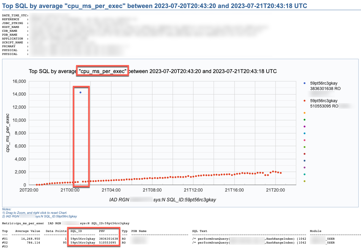

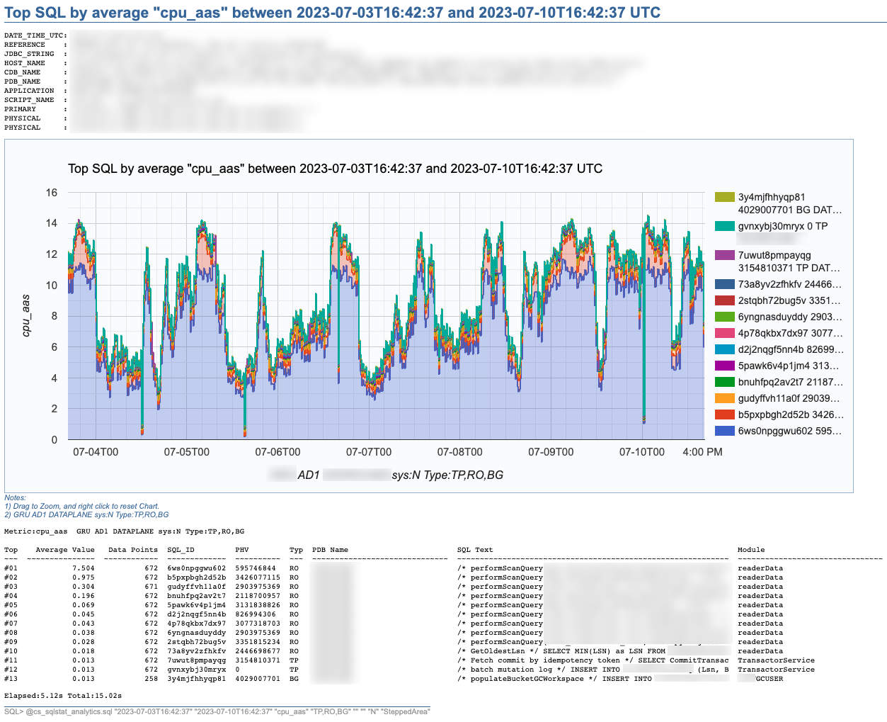
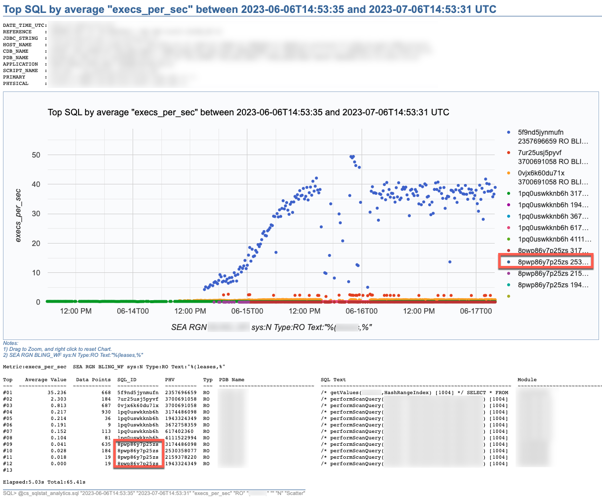
SQL Stats Analytics reads mainly DBA_HIST_SQLSTAT, performs some aggregations to compute multiple SQL statistics, selects the “top” SQL_ID/PLAN_HASH_VALUE pairs as per one selected Statistic, and produces some free Google chart, writing it into a text file to your local SQL*Plus directory where you started SQL*Plus (either on your Term client such as Mac/PC, or your DB server). The generated text file contains plain html, thus it can be opened using any browser. The chart allows some useful zooming on it.
On the “CS Scripts” README.md, you can find this SQL Statistics Analytics as well as its siblings (below). If you want to know what else is there on the “CS Scripts” Tool Set, simply navigate the readme. I do use many of these scripts on a daily basis, and I upload a fresh version to GitHub every so often.

These days I no longer consume SQLT, and I rarely use eDB360 or SQLdb360, since the “CS Scripts” Tool Set gives me everything I need on a piece-by-piece as-needed basis.
The SQL Stats Analytics takes the following input parameters:
- Time From (default to last 7 days)
- Time To (default to now)
- SQL Statistic (exhaustive list of 74 options where most common are: et_ms_per_exec default, et_aas, execs_per_sec, gets_per_exec and rows_per_exec)
- SQL Type (optional SQL categorization, but you may want to just skip this parameter)
- SQL Text piece (optional and case insensitive)
- SQL_ID (optional)
- Include SYS SQL (default to N)
- Graph Type (Scatter default, Line, SteppedArea and Area)
When using the “SQL Text piece” parameter you can focus on a set of SQL statements on a particular application Table, or maybe a SQL predicate of interest. The range of time is limited to your AWR retention (we keep 60 days of history and 15 minutes granularity since defaults of 8 days and 1 hour are not enough for our needs).
If you like this SQL Statistics Analytics script, you may also like the CS Ash Analytics. The former focuses on SQL Performance out of V$SQLSTATS while the latter on SQL Load out of V$ACTIVE_SESSION_HISTORY (and their DBA_HIST views).
Before using any of the CS Scripts, just be sure you are licensed on the Oracle Diagnostics Pack. Be also aware some scripts also use functionality covered under the Oracle Tuning Pack. And as with any other script you download from the internet, please read-proof it entirely and validate its proper use on your site.
Hope you get to enjoy the “CS Scripts” Tool Set!
Scripts to deal with SQL Plan Baselines, SQL Profiles and SQL Patches
To mitigate SQL performance issues, I do make use of SQL Plan Baselines, SQL Profiles and SQL Patches, on a daily basis. Our environments are single-instance 12.1.0.2 CDBs, with over 2,000 PDBs. Our goal is Execution Plan Stability and consistent performance, over CBO plan flexibility. The CBO does a good job, considering the complexity imposed by current applications design. Nevertheless, some SQL require some help in order to enhance their plan stability.
I have written and shared a set of scripts that simply make the use of a bunch of APIs a lot easier, with better documented actions, and fully consistent within the organization. I have shared with the community these scripts in the past, and I keep them updated as per needs change. All these “CS” scripts are available under the download section on the right column.
Current version of the CS scripts is more like a toolset. You treat them as a whole. All of them call some other script that exists within the cs_internal subdirectory, then I usually navigate to the parent sql directory, and connect into SQL*Plus from there. All these scripts can be easily cloned and/or customized to your specific needs. They are available as “free to use” and “as is”. There is no requirement to keep their heading intact, so you can reverse-engineer them and make them your own if you want. Just keep in mind that I maintain, enhance, and extend this CS toolset every single day; so what you get today is a subset of what you will get tomorrow. If you think an enhancement you need (or a fix) is beneficial to the larger community (and to you), please let me know.
SQL Plan Baselines scripts
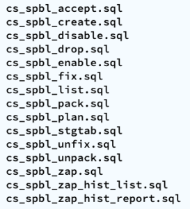
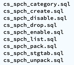
With the set of SQL Plan Baselines scripts, you can: 1) create a baseline based on a cursor or a plan stored into AWR; 2) enable and disable baselines; 3) drop baselines; 4) store them into a local staging table; 5) restore them from their local staging table; 6) promote as “fixed” or demote from “fixed”; 7) “zap” them if you have installed “El Zapper” (iod_spm).
Note: “El Zapper” is a PL/SQL package that extends the functionality of SQL Plan Management by automagically creating SQL Plan Baselines based on proven performance of a SQL statement over time, while considering a large number of executions, and a variety of historical plans. Please do not confuse “El Zapper” with auto-evolve of SPM. They are based on two very distinct premises. “El Zapper” also monitors the performance of active SQL Plan Baselines, and during an observation window it may disable a SQL Plan Baseline, if such plan no longer performs as “promised” (according to some thresholds). Most applications do not need “El Zapper”, since the use of SQL Plan Management should be more of an exception than a rule.
SQL Profiles scripts
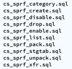
With the set of SQL Profiles scripts, you can: 1) create a profile based on the outline of a cursor, or from a plan stored into AWR; 2) enable and disable profiles; 3) drop profiles; 4) store them into a local staging table; 5) restore them from their local staging table; 6) transfer them from one location to another (very similar to coe_xfr_sql_profile.sql, but on a more modular way).
Note: Regarding the transfer of a SQL Profile, the concept is simple: 1) on source location generate two plain text scripts, one that contains the SQL text, and a second that includes the Execution Plan (outline); 2) execute these two scripts on a target location, in order to create a SQL Profile there. The beauty of this method is not only that you can easily move Execution Plans between locations, but that you can actually create a SQL Profile getting the SQL Text from SQL_ID “A”, and the Execution Plan from SQL_ID “B”, allowing you to do things like: removing CBO Hints, or using a plan from a similar SQL but not quite the same (e.g. I can tweak a stand-alone cloned version of a SQL statement, and once I get the plan that I need, I associate the SQL Text from the original SQL, with the desired Execution Plan out of the stand-alone customized version of the SQL, after that I create a SQL Plan Baseline and drop the staging SQL Profile).
SQL Patches scripts
With the set of SQL Patches scripts, you can: 1) create a SQL patch based on one or more CBO Hints you provide (e.g.: GATHER_PLAN_STATISTICS MONITOR FIRST_ROWS(1) OPT_PARAM(‘_fix_control’ ‘5922070:OFF’) NO_BIND_AWARE); 2) enable and disable SQL patches; 3) drop SQL patches; 4) store them into a local staging table; 5) restore them from their local staging table.
Note: I use SQL Patches a lot, specially to embed CBO Hints that generate some desirable diagnostics details (and not so much to change plans), such as the ones provided by GATHER_PLAN_STATISTICS and MONITOR. In some cases, after I use the pathfinder tool written by Mauro Pagano, I have to disable a CBO patch (funny thing: I use a SQL Patch to disable a CBO Patch!). I also use a SQL Patch if I need to enable Adaptive Cursor Sharing (ACS) for one SQL (we disabled ACS for one major application). Bear in mind that SQL Plan Baselines, SQL Profiles and SQL Patches happily co-exist, so you can use them together, but I do prefer to use SQL Plan Baselines alone, whenever possible.
Adapting and adopting SQL Plan Management (SPM)
Introduction
This post is about: “Adapting and adopting SQL Plan Management (SPM) to achieve execution plan stability for sub-second queries on a high-rate OLTP mission-critical application”. In our case, such an application is implemented on top of several Oracle 12c multi tenant databases, where a consistent average execution time is more valuable than flexible execution plans. We successfully achieved plan stability implementing a simple algorithm using PL/SQL calling DBMS_SPM public APIs.
Chart below depicts a typical case where the average performance of a large set of business-critical SQL statements suddenly degraded from sub-millisecond to 15 or 20ms, then beccome more stable around 3ms. Wide spikes are a typical trademark of an Execution Plan for one or more SQL statements flipping for some time. In order to produce a more consistent latency we needed to improve plan stability, and of course the preferred tool to achieve that on an Oracle database is SQL Plan Management.

Algorithm
We tested and ruled out adaptive SQL Plan Management, which is an excellent 12c new feature. But, due to the dynamics of this application, where transactional data shifts so fast, allowing this “adaptive SPM” feature to evaluate auto-captured plans using bind variable values captured a few hours earlier, rendered unfortunately false positives. These false positives “evolved” as execution plans that were numerically optimal for values captured (at the time the candidate plan was captured), but performed poorly when executed on “current” values a few hours later. Nevertheless, this 12c “adaptive SPM” new feature is worth exploring for other applications.
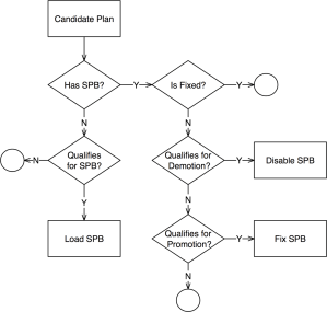 We adapted SPM so it would only generate SQL Plan Baselines on SQL that executes often, and that is critical for the business. The algorithm has some complexity such as candidate evaluation and SQL categorization; and besides SPB creation it also includes plan demotion and plan promotion. We have successfully implemented it in some PDBs and we are currently doing a rollout to entire CDBs. The algorithm is depicted on diagram on the left, and more details are included in corresponding presentation slides listed on the right-hand bar. I plan to talk about this topic on an international Oracle Users Group in 2018.
This algorithm is scripted into a sample PL/SQL package, which you can find on a subdirectory on my shared scripts. If you consider using this sample script for an application of your own, be sure you make it yours before attempting to use it. In other words: fully understand it first, then proceed to customize it accordingly and test it thoroughly.
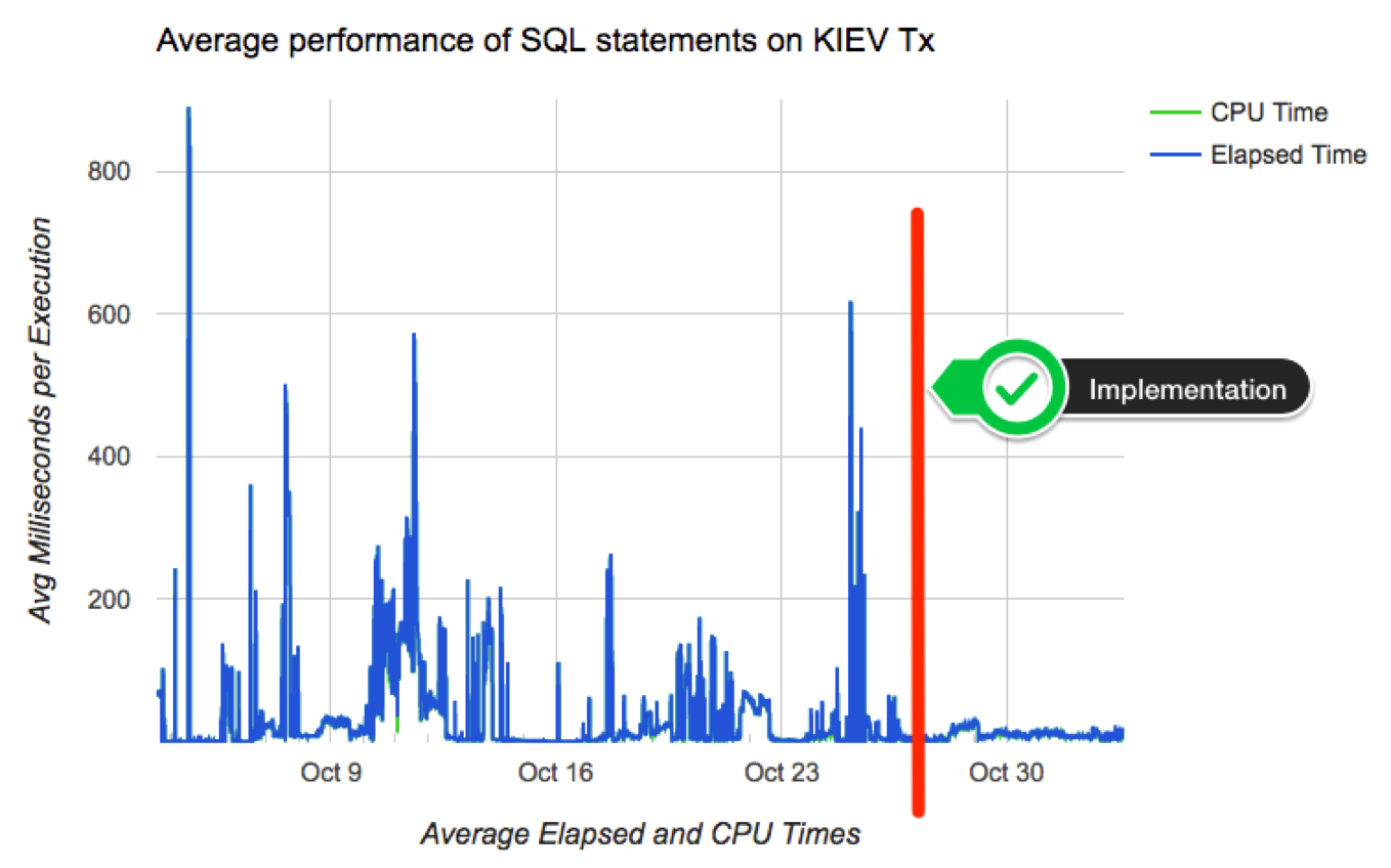
Results
Chart below shows how average performance of business-critical SQL became more stable after implementing algorithm to adapt and adopt SPM on a pilot PDB. Not all went fine although: we had some outliers that required some tuning to the algorithm. Among challenges we faced: volatile data (creating a SPB when table was almost empty, then using it when table was larger); skewed values (create a SPB for non-popular value, then using it on a popular value); proper use of multiple optimal plans due to Adaptive Cursor Sharing (ACS); rejected candidates due to conservative initial restrictions on algorithm (performance per execution, number of executions, age of cursor, etc.)
Conclusion
If your OLTP application contains business critical SQL that executes at a high-rate, and where a spike on latency risks affecting SLAs, you may want to consider implementing SQL Plan Management. Consider then both: “adaptive SPM” if it satisfies your requirements, else build a PL/SQL library that can implement more complex logic for candidates evaluation and for SPBs maintenance. I do believe SPM works great, specially when you enhance its out-of-the-box functionality to satisfy your specific needs.
SQL Monitoring without MONITOR Hint
I recently got this question:
<<<Is there a way that I can generate SQL MONITORING report for a particular SQL_ID ( This SQL is generated from application code so I can’t add “MONITOR” hint) from command prompt ? If yes can you please help me through this ?>>>
Since this question is of general interest, I’d rather respond here:
As you know, SQL Monitoring starts automatically on a SQL that executes a PX plan, or when its Serial execution has consumed over 5 seconds on CPU or I/O.
If you want to force SQL Monitoring on a SQL statement, without modifying the SQL text itself, I suggest you create a SQL Patch for it. But before you do, please be aware that SQL Monitoring requires the Oracle Tuning Pack.
How to turn on SQL Monitoring for a SQL that executes Serial, takes less than 5 seconds, and without modifying the application that issues such SQL
Use SQL Patch with the MONITOR Hint. An easy way to do that is by using the free sqlpch.sql script provided as part of the cscripts (see right-hand side of this blog under Downloads).
To use sqlpch.sql script, pass as parameter #1 your SQL_ID and for parameter #2 pass “GATHER_PLAN_STATISTICS MONITOR” (without the double quotes).
This sqlpch.sql script will create a SQL Patch for your SQL, which will produce SQL Monitoring (and the collection of A-Rows) for every execution of your SQL.
Be aware there is some overhead involved, so after you are done with your analysis drop the SQL Patch.
Script sqlpch.sql shows the name of the SQL Patch it creates (look at its spool file), and it gives you the command to drop such SQL Patch.
For the actual analysis and diagnostics of your SQL (after you have executed it with SQL Patch in place) use free tool SQLd360.
And for more details about sqlpch.sql and other uses of this script please refer to this entry on my blog.
Forcing a “Nested Loop only” Execution Plan
Sometimes you do what you have to do. So here I confess doing something I usually avoid: forcing an Execution Plan (which is not the same as using a more conventional method for Plan stability).
This is a case on 11.2.0.3.0 base release where the application vendor sets the optimizer to 9i, and tweaks other CBO parameters in questionable ways, then some queries produce suboptimal plans (as expected); and you are called to help without changing the obvious.
There is a family of queries from an ad-hoc query generator that permits users to issue queries without a set of selective predicates. These queries join several large tables and their performance is poor (as expected as well!). On top of the previous, all these queries include the /*+ FIRST_ROWS */ CBO Hint and the questionable DISTINCT keyword. Note: it is quite common for developers to throw a DISTINCT keyword “to avoid duplicates” where the mere existence of duplicates would be an indication of an application bug; so “why fix it if I can hide it, right?”.
There is one caveat although: these queries include a generic predicate “rownum <= :b1”, and value passed defaults to 5000, so users rationale is “if I only want the first X rows my query should return fast”. This highlights still another questionable practice since it is hard to imagine a user scrolling 5000 rows and making any sense of such large set, especially when the full “filtered” set would be several million rows long. So the original problem is questionable in several ways. Nevertheless, sometimes we are called to help besides providing advice. And no, we are not allowed to slap hands 😉
The good news is that we can use this extra predicate on rownum and make these queries to return the first X rows really fast; and I mean less than 5 seconds instead of over one hour or more! And if users want not 5000 but 500 or even 50 rows, then we can be in the sub-second range!
You may be thinking FIRST_ROWS optimization, and that was my first try. Unfortunately, on 11.2.0.3.0, even reversing all the suboptimal CBO parameters at the session level, I would consistently get an Execution Plan with a few Hash Joins and a large Cost; and if I were to force a Nested Loop Plan, the cost would be several orders of magnitude larger so the CBO would not pick it! Nevertheless, such a “Nest Loop only” Execution Plan would fulfill the user’s expectations, regardless the validity of the initial request. And yes, CBO statistics are OK, not perfect but simply OK. One more piece of info: this is not Exadata! (if it were Exadata most probably these same Execution Plans with full table scans and Hash Joins would simply fly!).
So, my issue became: How do I force an Execution Plan that only contains Nested Loops? If I could do that, then the COUNT STOP operation could help me to halt my SQL execution once I fetched the first X rows (Hash Join does not allow me do that). Remember: these tables have literally millions of rows. I could pepper these queries with a ton of CBO Hints and I would get my desired “Nested Loop only” Execution Plan… But that would be a lot of work and tricky at best.
SQL Patch to the rescue
I could had used a SQL Profile, but I think this dirty trick of suppressing Hash Joins and Sort Merge Joins, would be better served with a SQL Patch. I also thought Siebel: They do tweak CBO parameters as well, and they suppress Hash Joins, but they change System and Session level parameters… Since I wanted my change to be very localized, SQL Patch could provide me just what I needed.
Under the Downloads section on the margin of this page, there is a “cscripts” link that includes the sqlpch.sql script. I used this script and passed as the second parameter the following string (1st parameter is SQL_ID). With a SQL Patch generated this way, I could systematically produce a “Nested-Loops only” Execution Plan for these few queries. I did not have to change the original SQL, nor change the CBO environment at the System or Session level, neither restrict the query generator, and I did not had to “educate” the users to avoid such unbounded queries.
OPT_PARAM("_optimizer_sortmerge_join_enabled" "FALSE") OPT_PARAM("_hash_join_enabled" "FALSE")
Conclusion
I have to concede doing something questionable, in this case using a SQL Patch to force a desired Execution Plan instead of fixing the obvious, simply because that was the shortest path to alleviate the user’s pain.
I consider this technique above a temporary work-around and not a solution to the actual issue. In this case the right way to handle this issue would be:
- Have the application vendor certify their application to the latest release of the database and reset all CBO related parameters, plus
- Have the application vendor remove CBO Hints and DISTINCT keyword from queries, plus
- Configure the ad-hoc query generator to restrict users from executing queries without selective predicates, then
- Tune those outlier queries that may still need some work to perform as per business requirements, and possibly
- Educate the users to provide as many selective predicates as possible
Anyways, the potential of using a SQL Patch to tweak an Execution Plan in mysterious ways is quite powerful, and something we may want to keep in the back of our minds for a rainy day…
edb360 taking a long time
In most cases edb360 takes less than 1hr to execute. But I often hear of cases where it takes a lot longer than that. In a corner case it was taking several days and it had to be killed.
So the question is WHY edb360 takes that long?
Well, edb360 executes thousands of SQL statements sequentially (intentionally). Many of these queries read data from AWR and in particular from ASH. So, lets say your ASH historical table has 2B rows, and on top of that you have not gathered statistics on AWR tables in years, thus CBO under-estimates cardinality and tends to use index access and nested loops. In such extreme cases you may end up with suboptimal execution plans that expect to return a few rows, but actually read a couple of billion rows using index access operations and nested loops. A query like this may take hours to complete!
As of version v1515, edb360 has a shortcut algorithm that ends an execution after 8 hours. So you may get an incomplete output, but it ends normally and the partial output can actually be used. This is not a solution but a workaround for those long executions.
How to troubleshoot edb360 taking long?
Steps:
1. Review files 00002_edb360_dbname_log.txt, 00003_edb360_dbname_log2.txt, 00004_edb360_dbname_log3.txt and 00005_edb360_dbname_tkprof_sort.txt. First log shows the state of the statistics for AWR Tables. If stats are old then gather them fresh with script edb360/sql/gather_stats_wr_sys.sql
2. If number of rows on WRH$_ACTIVE_SESSION_HISTORY as per 00002_edb360_dbname_log.txt is several millions, then you may not be purging data periodically. There are some known bugs and some blog posts on this regard. Review MOS 387914.1 and proceed accordingly. Execute query below to validate ASH age:
SELECT TRUNC(sample_time, 'MM'), COUNT(*)
  FROM dba_hist_active_sess_history
 GROUP BY TRUNC(sample_time, 'MM')
 ORDER BY TRUNC(sample_time, 'MM')
 /
3. If edb360 version (first line on its readme) is older than 1 month, download and use latest version: https://github.com/carlos-sierra/edb360/archive/master.zip (link is also provided on the right-hand side of this blog under downloads).
4. Consider suppressing text and or csv reports. Each for an estimated gain of about 20%. Keep in mind that when suppressing reports, you start loosing some functionality. To suppress lets say text and csv reports, place the following two commands at the end of script edb360/sql/edb360_00_config.sql
DEF edb360_conf_incl_text = ‘N’;
DEF edb360_conf_incl_csv = ‘N’;
5. If after going through steps 1-4 above, edb360 still takes longer than a few hours, feel free to email author carlos.sierra.usa@gmail.com and provide 4 files from step 1.
Discovering if a System level Parameter has changed its value (and when it happened)
Quite often I learn of a system where “nobody changed anything” and suddenly the system is experiencing some strange behavior. Then after diligent investigation it turns out someone changed a little parameter at the System level, but somehow disregarded mentioning it since he/she thought it had no connection to the unexpected behavior. As we all know, System parameters are big knobs that we don’t change lightly, still we often see “unknown” changes like the one described.
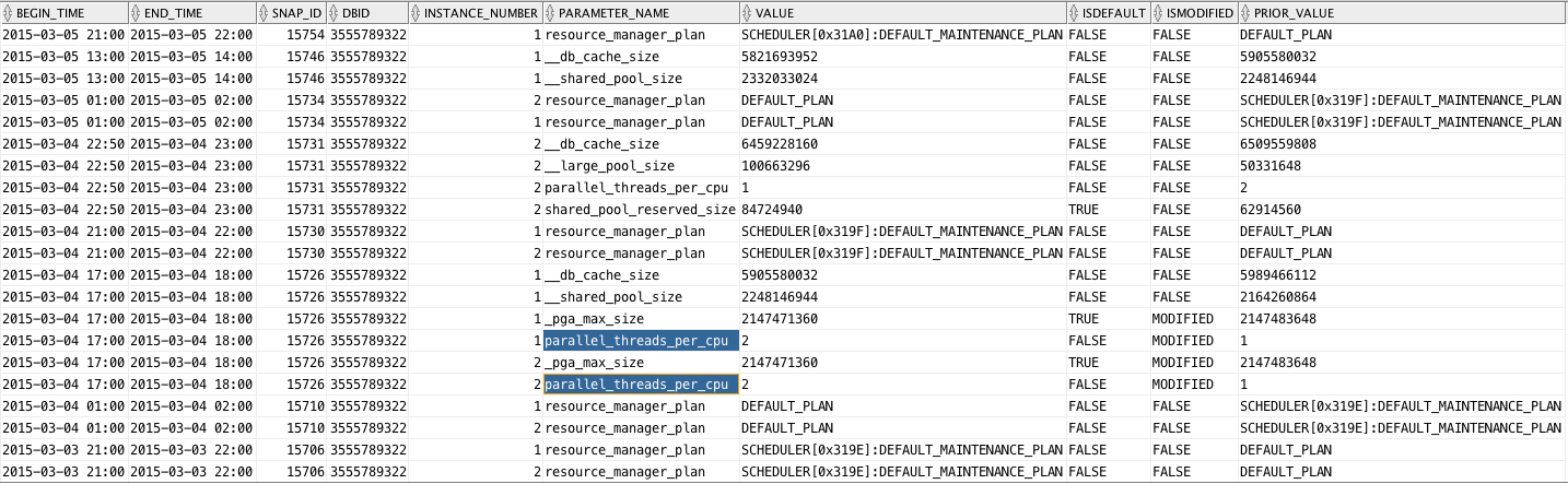
Script below produces a list of changes to System parameter values, indicating when a parameter was changed and from which value into which value. It does not filter out cache re-sizing operations, or resource manager plan changes. Both would be easy to exclude, but I’d rather see those global changes listed as well.
Note: This script below should only be executed if your site has a license for the Oracle Diagnostics pack (or Tuning pack), since it reads from AWR.
WITH
all_parameters AS (
SELECT snap_id,
       dbid,
       instance_number,
       parameter_name,
       value,
       isdefault,
       ismodified,
       lag(value) OVER (PARTITION BY dbid, instance_number, parameter_hash ORDER BY snap_id) prior_value
  FROM dba_hist_parameter
)
SELECT TO_CHAR(s.begin_interval_time, 'YYYY-MM-DD HH24:MI') begin_time,
       TO_CHAR(s.end_interval_time, 'YYYY-MM-DD HH24:MI') end_time,
       p.snap_id,
       p.dbid,
       p.instance_number,
       p.parameter_name,
       p.value,
       p.isdefault,
       p.ismodified,
       p.prior_value
  FROM all_parameters p,
       dba_hist_snapshot s
 WHERE p.value != p.prior_value
   AND s.snap_id = p.snap_id
   AND s.dbid = p.dbid
   AND s.instance_number = p.instance_number
 ORDER BY
       s.begin_interval_time DESC,
       p.dbid,
       p.instance_number,
       p.parameter_name
/
Sample output follows, where we can see a parameter affecting Degree of Parallelism was changed. This is just to illustrate its use. Enjoy this new free script! It is now part of edb360.
SQLTXPLAIN under new administration
During my 17 years at Oracle, I developed several tools and scripts. The largest and more widely used is SQLTXPLAIN. It is available through My Oracle Support (MOS) under document_id 215187.1.
SQLTXPLAIN, also know as SQLT, is a tool for SQL diagnostics, including Performance and Wrong Results. I am the original developer and author, but since very early stages of its development, this tool encapsulates the expertise of many bright engineers, DBAs, developers and others, who constantly helped to improve this tool on every new release by providing valuable feedback. SQLT is then nothing but the collection of many good ideas from many people. I was just the lucky guy that decided to build something useful for the Oracle SQL tuning community.
When I decided to join Enkitec back on 2013, I asked Mauro Pagano to look after my baby (I mean SQLT), and sure enough he did an excellent job. Mauro fixed most of my bugs, as he jokes about, and also incorporated some of his own :-). Mauro kept SQLT in good shape and he was able to continue improving it on every new release. Now Mauro also works for Enkitec, so SQLT has a new owner and custodian at Oracle.
Abel Macias is the new owner of SQLT, and as such he gets busy maintaining and enhancing this tool among other duties at Oracle. So, if you have enhancement requests, or positive feedback, please reach out to Abel at his Oracle account: abel.macias@oracle.com. If you come across some of my other tools and scripts, and they show my former Oracle account (carlos.sierra@oracle.com), please reach out to Abel and he might be able to route your concern or question.
Since one of my hobbies is to build free software that I also consume, my current efforts are on eDB360, eAdam and eSP. The most popular and openly available is eDB360, which basically gives your a 360-degree view of a database without installing anything. Then, Mauro is also building something cool on his own free time. Mauro is building the new SQLd360 tool, which is already available on the web (search for SQLd360). This SQLd360 tool, similar to eDB360, provides a 360-degree view, but instead of a database its focus is one SQL. And similarly than eDB360 it installs nothing on the database. Both are available as “free software” for anyone to download and use. That is the nice part: everyone likes free! (specially if any good).
What is the difference between SQLd360 and SQLT?
Both are exceptional tools. And both can be used for SQL Tuning and for SQL diagnostics. The main differences in my opinion are these:
- SQLT has it all. It is huge and it covers pretty much all corners. So, for SQL Tuning this SQLTXPLAIN is “THE” tool.
- SQLd360 in the other hand is smaller, newer and faster to execute. It gives me what is more important and most commonly used.
- SQLT requires to install a couple of schemas and hundreds of objects. SQLd360 installs nothing!
- To download SQLT you need to login into MOS. In contrast, SQLd360 is wide open (free software license), and no login is needed.
- Oracle Support requires SQLT, and Oracle Engineers are not exposed yet to SQLd360.
- SQLd360 uses Google charts (as well as eDB360 does) which enhance readability of large data sets, like time series for example. Thus SQLd360 output is quite readable.
- eDB360 calls SQLd360 on SQL of interest (large database consumers), so in that sense SQLd360 enhances eDB360. But SQLd360 can also be used stand-alone.
If you ask me which one would I recommend, I would answer: both!. If you can use both, then that is better than using just one. Each of these two tools (SQLT and SQLd360) has pros and cons compared to the other. But at the end both are great tools. And thanks to Abel Macias, SQLT continues its lifecycle with frequent enhancements. And thanks to Mauro, we have now a new kid on the block! I would say we have a win-win for our large Oracle community!
Free script to generate a Line Chart on HTML
Performance Metrics are easier to digest if visualized trough some Line Charts. OEM, eDB360, eAdam and other tools use them. If you already have a SQL Statement that provides the Performance Metrics you care about, and just need to generate a Line Chart for them, you can easily create a CSV file and open it with MS-Excel. But if you want to build an HTML Report out of your SQL, that is a bit harder, unless you use existing technologies. Tools like eDB360 and eAdam use Google Charts as a mechanism to easily generate such Charts. A peer asked me if we could have such functionality stand-alone, and that challenged me to create and share it.
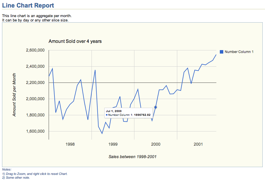
This HTML Line Chart Report above was created with script line_chart.sql shown below. The actual chart, which includes Zoom functionality on HTML can be downloaded from this Dropbox location. Feel free to use this line_chart.sql script as a template to display your Performance Metrics. It can display several series into one Chart (example above shows only one), and by reviewing code below you will find out how easy it is to adjust to your own needs. Chart above was created using a simple query against the Oracle Sample Schema SH, but the actual use could be Performance Metrics or any other Application time series.
Script
SET TERM OFF HEA OFF LIN 32767 NEWP NONE PAGES 0 FEED OFF ECHO OFF VER OFF LONG 32000 LONGC 2000 WRA ON TRIMS ON TRIM ON TI OFF TIMI OFF ARRAY 100 NUM 20 SQLBL ON BLO . RECSEP OFF;
PRO
DEF report_title = "Line Chart Report";
DEF report_abstract_1 = "<br>This line chart is an aggregate per month.";
DEF report_abstract_2 = "<br>It can be by day or any other slice size.";
DEF report_abstract_3 = "";
DEF report_abstract_4 = "";
DEF chart_title = "Amount Sold over 4 years";
DEF xaxis_title = "Sales between 1998-2001";
--DEF vaxis_title = "Amount Sold per Hour";
--DEF vaxis_title = "Amount Sold per Day";
DEF vaxis_title = "Amount Sold per Month";
DEF vaxis_baseline = ", baseline:2200000";
DEF chart_foot_note_1 = "<br>1) Drag to Zoom, and right click to reset Chart.";
DEF chart_foot_note_2 = "<br>2) Some other note.";
DEF chart_foot_note_3 = "";
DEF chart_foot_note_4 = "";
DEF report_foot_note = "This is a sample line chart report.";
PRO
SPO line_chart.html;
PRO <html>
PRO <!-- $Header: line_chart.sql 2014-07-27 carlos.sierra $ -->
PRO <head>
PRO <title>line_chart.html</title>
PRO
PRO <style type="text/css">
PRO body   {font:10pt Arial,Helvetica,Geneva,sans-serif; color:black; background:white;}
PRO h1     {font-size:16pt; font-weight:bold; color:#336699; border-bottom:1px solid #cccc99; margin-top:0pt; margin-bottom:0pt; padding:0px 0px 0px 0px;}
PRO h2     {font-size:14pt; font-weight:bold; color:#336699; margin-top:4pt; margin-bottom:0pt;}
PRO h3     {font-size:12pt; font-weight:bold; color:#336699; margin-top:4pt; margin-bottom:0pt;}
PRO pre    {font:8pt monospace;Monaco,"Courier New",Courier;}
PRO a      {color:#663300;}
PRO table  {font-size:8pt; border_collapse:collapse; empty-cells:show; white-space:nowrap; border:1px solid #cccc99;}
PRO li     {font-size:8pt; color:black; padding-left:4px; padding-right:4px; padding-bottom:2px;}
PRO th     {font-weight:bold; color:white; background:#0066CC; padding-left:4px; padding-right:4px; padding-bottom:2px;}
PRO td     {color:black; background:#fcfcf0; vertical-align:top; border:1px solid #cccc99;}
PRO td.c   {text-align:center;}
PRO font.n {font-size:8pt; font-style:italic; color:#336699;}
PRO font.f {font-size:8pt; color:#999999; border-top:1px solid #cccc99; margin-top:30pt;}
PRO </style>
PRO
PRO <script type="text/javascript" src="https://www.google.com/jsapi"></script>
PRO <script type="text/javascript">
PRO google.load("visualization", "1", {packages:["corechart"]})
PRO google.setOnLoadCallback(drawChart)
PRO
PRO function drawChart() {
PRO var data = google.visualization.arrayToDataTable([
/* add below more columns if needed (modify 3 places) */
PRO ['Date Column', 'Number Column 1']
/****************************************************************************************/
WITH
my_query AS (
/* query below selects one date_column and a small set of number_columns */
SELECT --TRUNC(time_id, 'HH24') date_column /* preserve the column name */
       --TRUNC(time_id, 'DD') date_column /* preserve the column name */
       TRUNC(time_id, 'MM') date_column /* preserve the column name */
       , SUM(amount_sold) number_column_1 /* add below more columns if needed (modify 3 places) */
  FROM sh.sales
 GROUP BY
       --TRUNC(time_id, 'HH24') /* aggregate per hour, but it could be any other */
       --TRUNC(time_id, 'DD') /* aggregate per day, but it could be any other */
       TRUNC(time_id, 'MM') /* aggregate per month, but it could be any other */
/* end of query */
)
/****************************************************************************************/
/* no need to modify the date column below, but you may need to add some number columns */
SELECT ', [new Date('||
       TO_CHAR(q.date_column, 'YYYY')|| /* year */
       ','||(TO_NUMBER(TO_CHAR(q.date_column, 'MM')) - 1)|| /* month - 1 */
       --','||TO_CHAR(q.date_column, 'DD')|| /* day */
       --','||TO_CHAR(q.date_column, 'HH24')|| /* hour */
       --','||TO_CHAR(q.date_column, 'MI')|| /* minute */
       --','||TO_CHAR(q.date_column, 'SS')|| /* second */
       ')'||
       ','||q.number_column_1|| /* add below more columns if needed (modify 3 places) */
       ']'
  FROM my_query q
 ORDER BY
       date_column
/
/****************************************************************************************/
PRO ]);
PRO
PRO var options = {
PRO backgroundColor: {fill: '#fcfcf0', stroke: '#336699', strokeWidth: 1},
PRO explorer: {actions: ['dragToZoom', 'rightClickToReset'], maxZoomIn: 0.1},
PRO title: '&&chart_title.',
PRO titleTextStyle: {fontSize: 16, bold: false},
PRO focusTarget: 'category',
PRO legend: {position: 'right', textStyle: {fontSize: 12}},
PRO tooltip: {textStyle: {fontSize: 10}},
PRO hAxis: {title: '&&xaxis_title.', gridlines: {count: -1}},
PRO vAxis: {title: '&&vaxis_title.' &&vaxis_baseline., gridlines: {count: -1}}
PRO }
PRO
PRO var chart = new google.visualization.LineChart(document.getElementById('chart_div'))
PRO chart.draw(data, options)
PRO }
PRO </script>
PRO </head>
PRO <body>
PRO <h1>&&report_title.</h1>
PRO &&report_abstract_1.
PRO &&report_abstract_2.
PRO &&report_abstract_3.
PRO &&report_abstract_4.
PRO <div id="chart_div" style="width: 900px; height: 500px;"></div>
PRO <font class="n">Notes:</font>
PRO <font class="n">&&chart_foot_note_1.</font>
PRO <font class="n">&&chart_foot_note_2.</font>
PRO <font class="n">&&chart_foot_note_3.</font>
PRO <font class="n">&&chart_foot_note_4.</font>
PRO <pre>
L
PRO </pre>
PRO <br>
PRO <font class="f">&&report_foot_note.</font>
PRO </body>
PRO </html>
SPO OFF;
SET HEA ON LIN 80 NEWP 1 PAGES 14 FEED ON ECHO OFF VER ON LONG 80 LONGC 80 WRA ON TRIMS OFF TRIM OFF TI OFF TIMI OFF ARRAY 15 NUM 10 NUMF "" SQLBL OFF BLO ON RECSEP WR;
SQLTXPLAIN PL/SQL Public APIs to execute XTRACT from 3rd party tools
Many tools offer Public APIs, which expose some functionality to other tools. SQLTXPLAIN contains also some Public APIs. They are provided by package SQLTXADMIN.SQLT$E. I would say the most relevant one is XTRACT_SQL_PUT_FILES_IN_DIR. This blog post is about this Public API and how it can be used by other tools to execute a SQLT XTRACT from PL/SQL instead of SQL*Plus.
Imagine a tool that deals with SQL statements, and with the click of a button it invokes SQLTXTRACT on a SQL of interest, and after a few minutes, most files created by SQLTXTRACT suddenly show on an OS pre-defined directory. Implementing this SQLT functionality on an external tool is extremely easy as you will see below.
Public API SQLTXADMIN.SQLT$E.XTRACT_SQL_PUT_FILES_IN_DIR inputs a SQL_ID and two other optional parameters: A tag to identify output files, and a directory name. Only SQL_ID parameter is mandatory, and the latter two are optional, but I recommend to pass values for all 3.
I used “Q1” as a tag to be included in all output files. And I used staging directory “FROG_DIR” at the database layer, which points to “/home/oracle/frog” at the OS layer.
On sample below, I show how to use this Public API for a particular SQL_ID “8u0n7w1jug5dg”. I call this API from SQL*Plus, but keep in mind that if I were to call it from within a tool’s PL/SQL library, the method would be the same.
Another consideration is that Public API SQLTXADMIN.SQLT$E.XTRACT_SQL_PUT_FILES_IN_DIR may take several minutes to execute, so you may want to “queue” the request using a Task or a Job within the database. What is important here on this blog post is to explain and show how this Public API works.
SQLTXADMIN.SQLT$E.XTRACT_SQL_PUT_FILES_IN_DIR parameters:
Find below code snippet showing API Parameters. Notice this API is overloaded, so it may return the STATEMENT_ID or nothing. This STATEMENT_ID is the 5 digits number you see on each SQLT execution.
CREATE OR REPLACE PACKAGE &&tool_administer_schema..sqlt$e AUTHID CURRENT_USER AS
/* $Header: 215187.1 sqcpkge.pks 12.1.03 2013/10/10 carlos.sierra mauro.pagano $ */

  /*************************************************************************************/

  /* -------------------------
   *
   * public xtract_sql_put_files_in_dir
   *
   * executes sqlt xtract on a single sql then
   * puts all generated files into an os directory,
   * returning the sqlt statement id.
   *
   * ------------------------- */
  FUNCTION xtract_sql_put_files_in_dir (
    p_sql_id_or_hash_value IN VARCHAR2,
    p_out_file_identifier  IN VARCHAR2 DEFAULT NULL,
    p_directory_name       IN VARCHAR2 DEFAULT 'SQLT$STAGE' )
  RETURN NUMBER;

  /* -------------------------
   *
   * public xtract_sql_put_files_in_dir (overload)
   *
   * executes sqlt xtract on a single sql then
   * puts all generated files into an os directory.
   *
   * ------------------------- */
  PROCEDURE xtract_sql_put_files_in_dir (
    p_sql_id_or_hash_value IN VARCHAR2,
    p_out_file_identifier  IN VARCHAR2 DEFAULT NULL,
    p_directory_name       IN VARCHAR2 DEFAULT 'SQLT$STAGE' );
Staging Directory
To implement Public API SQLTXADMIN.SQLT$E.XTRACT_SQL_PUT_FILES_IN_DIR on your tool, you need first to create and test a staging directory where the API will write files. This directory needs to be accessible to the “oracle” account, so I show below how to create sample directory “frog” while connected to the OS as “oracle”.
Since the API uses UTL_FILE, it is important that “oracle” can write into it, so be sure you test this UTL_FILE write after you create the directory and before you test Public API SQLTXADMIN.SQLT$E.XTRACT_SQL_PUT_FILES_IN_DIR.
Use code snippet provided below to test the UTL_FILE writing into this new staging OS directory.
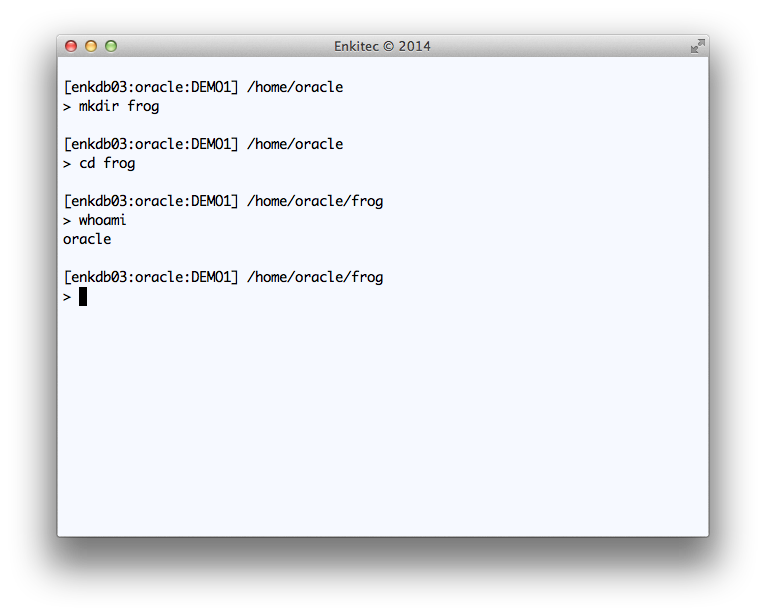
Creating “frog” OS directory connected to OS as “oracle”
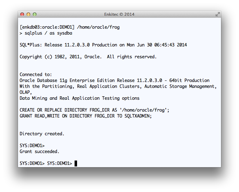
Creating FROG_DIR database directory and providing access to SQLTXADMIN
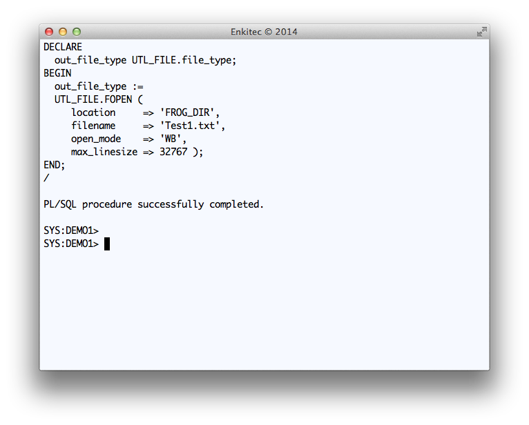
Testing a simple WRITE to FROG_DIR
DECLARE
  out_file_type UTL_FILE.file_type;
BEGIN
  out_file_type :=
  UTL_FILE.FOPEN (
     location     => 'FROG_DIR',
     filename     => 'Test1.txt',
     open_mode    => 'WB',
     max_linesize => 32767 );
END;
/
Executing SQLTXADMIN.SQLT$E.XTRACT_SQL_PUT_FILES_IN_DIR
On your tool, you can call this SQLT Public API from PL/SQL. You may want to use a Task or Job since the API may take several minutes to execute and you do not want the user to simply wait until SQLT completes.
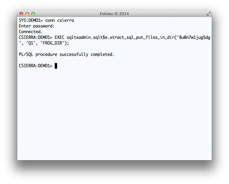
Execution of Public API SQLTXADMIN.SQLT$E.XTRACT_SQL_PUT_FILES_IN_DIR
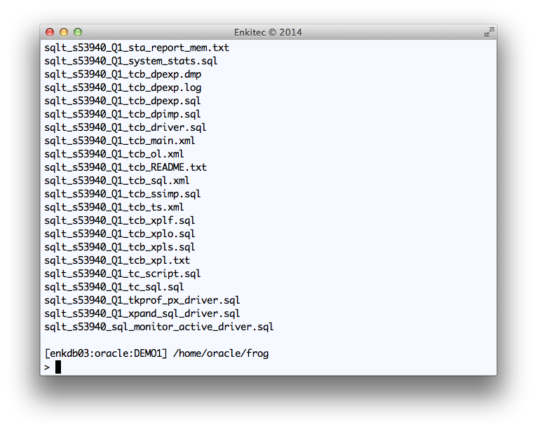
Reviewing the output of SQLT XTRACT for SQL_ID “8u0n7w1jug5dg”
Conclusion
Public API SQLTXADMIN.SQLT$E.XTRACT_SQL_PUT_FILES_IN_DIR is available for any 3rd party tool to use. If SQLT has been pre-installed on a system where your tool executes, then calling this API as shown above, will generate a set of SQLT files on a pre-defined staging OS directory.
If the system where you install your tool does not have SQLT pre-installed, your tool can direct its users to download and install SQLT out of My Oracle Support (MOS) under document 215187.1.
Once you generate all these SQLT XTRACT files into an OS staging directory, you may want to zip them, or make them visible to your tool user. If the latter, then show the “main” html report.
SQLT is an Oracle community tool hosted at Oracle MOS under 215187.1. This tool is not supported, but if you have a question or struggle while implementing this Public API, feel free to shoot me an email or post your question/concern on this blog.
