SQL Stats Analytics (from SQL*Plus!)
If you have access to some other graphical tool that displays time series on multiple dimensions for one or a set of SQL statements from an Oracle database, then you may not need “SQL Stats Analytics”. In the other hand, if you have no such tool, or even more restricting, if you can only access your Oracle database through some client connection such as SQL*Plus, then you may have some use for the open-source “SQL Stats Analytics” presented here.
Before you go on, a fair warning: this open-source tool reads DBA_HIST_SQLSTAT, therefore it assumes you are licensed to use the Oracle Diagnostics Pack, like when you access any DBA_HIST view. And a second caveat, this tool has been developed and tested on Oracle databases 12.2 and 19c, so it won’t work on older releases. Final note here: SQL Stats Analytics is part of the “CS Scripts” Tool Set (open-source), then you can use any of these scripts “as is”, but they are not actually supported by me or anyone else (they do work although). Feel free to use this part, or any other part of the “CS Scripts” Tool Kit at your own risk, and with the condition that you cannot claim authorship or ownership.
SQL Stats Analytics, similar to the “Poor-man’s version of ASH Analytics” presented on this blog, is a tool to generate, out of a simple SQL*Plus connection (either from a DB server or from a client machine: i.e.: a Term on a Mac or PC), a Chart that provide valuable insights on performance history and patterns, on one or multiple SQL statements of interest. Since a picture is worth a thousand words, I’d rather show some pictures, then explain briefly this tool.

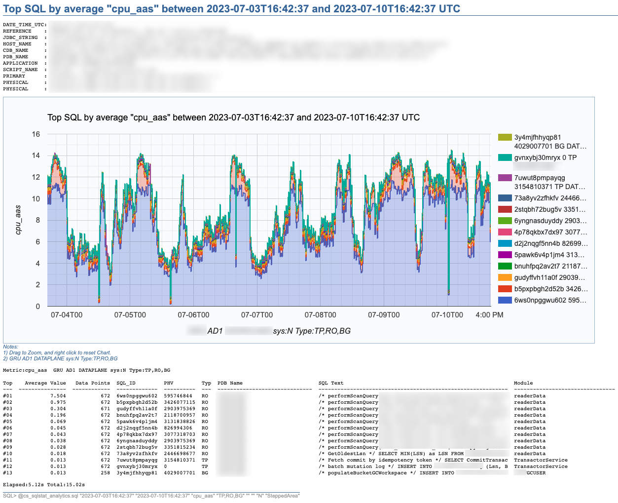
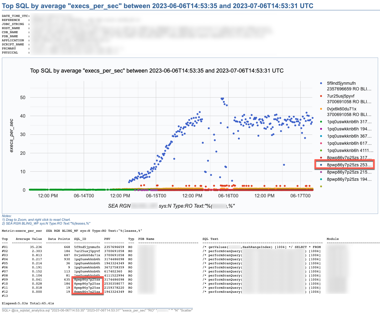
SQL Stats Analytics reads mainly DBA_HIST_SQLSTAT, performs some aggregations to compute multiple SQL statistics, selects the “top” SQL_ID/PLAN_HASH_VALUE pairs as per one selected Statistic, and produces some free Google chart, writing it into a text file to your local SQL*Plus directory where you started SQL*Plus (either on your Term client such as Mac/PC, or your DB server). The generated text file contains plain html, thus it can be opened using any browser. The chart allows some useful zooming on it.
On the “CS Scripts” README.md, you can find this SQL Statistics Analytics as well as its siblings (below). If you want to know what else is there on the “CS Scripts” Tool Set, simply navigate the readme. I do use many of these scripts on a daily basis, and I upload a fresh version to GitHub every so often.

These days I no longer consume SQLT, and I rarely use eDB360 or SQLdb360, since the “CS Scripts” Tool Set gives me everything I need on a piece-by-piece as-needed basis.
The SQL Stats Analytics takes the following input parameters:
- Time From (default to last 7 days)
- Time To (default to now)
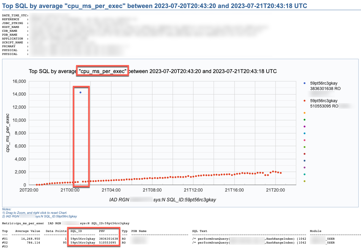
- SQL Statistic (exhaustive list of 74 options where most common are: et_ms_per_exec default, et_aas, execs_per_sec, gets_per_exec and rows_per_exec)
- SQL Type (optional SQL categorization, but you may want to just skip this parameter)
- SQL Text piece (optional and case insensitive)
- SQL_ID (optional)
- Include SYS SQL (default to N)
- Graph Type (Scatter default, Line, SteppedArea and Area)
When using the “SQL Text piece” parameter you can focus on a set of SQL statements on a particular application Table, or maybe a SQL predicate of interest. The range of time is limited to your AWR retention (we keep 60 days of history and 15 minutes granularity since defaults of 8 days and 1 hour are not enough for our needs).
If you like this SQL Statistics Analytics script, you may also like the CS Ash Analytics. The former focuses on SQL Performance out of V$SQLSTATS while the latter on SQL Load out of V$ACTIVE_SESSION_HISTORY (and their DBA_HIST views).
Before using any of the CS Scripts, just be sure you are licensed on the Oracle Diagnostics Pack. Be also aware some scripts also use functionality covered under the Oracle Tuning Pack. And as with any other script you download from the internet, please read-proof it entirely and validate its proper use on your site.
Hope you get to enjoy the “CS Scripts” Tool Set!
ASH Analytics from SQL*Plus
I used to like (Average Active Session History) ASH Analytics available trough Oracle Enterprise Manager (OEM). Then OEM was not always available, or the time to reach it was too long, or its access too cumbersome at best. Slowly for surely, I started using (and developing) stand-alone scripts to get what I needed from ASH in a timely manner.
Many Developers and even DBAs have access to an Oracle database through SQL*Plus, but not to OEM or any other GUI to check on database performance. And in many cases, access is only available through a client machine (i.e. your Mac or PC), but never to the actual database server directly.
If your site has an Oracle Diagnostics Pack License (i.e. you are authorized to access AWR and ASH data), then you can query your ASH data through SQL*Plus and generate some text-based reports. But, if you’d rather do your analysis visualizing your performance data through time-based charts, you could use tools such as SQLdb360, or some stand-alone scripts that execute on SQL*Plus (client or server-side) and produce charts like the one below. Note that such tools and scripts query AWR and ASH data.
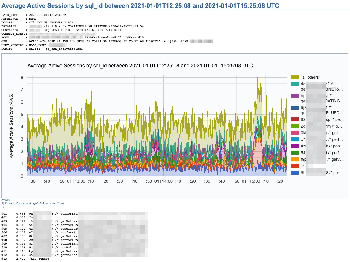
This chart above was produced by what I call “a poor’s man ASH analytics”. It gives me what I need in order to make an initial performance assessment in just a few minutes. It also allows me to properly document cases. This script cs_ash_analytics.sql is part of a subset of the “CS scripts“, available to download and use “as is” for free. Just be aware that many of these scripts should only be used if your site has a License for the Oracle Diagnostics or Tuning Packs. I use the “CS scripts” on a daily basis. And I update them every so often.
This one “ASH analytics” script, when executed from SQL*Plus, allows you to generate a time-based chart on recent (V$) or more persistent (DBA_HIST) ASH data. It provides for diverse dimension options such as: Wait Class, Event, Machine, SQL_ID, Plan Hash Value, Top Level SQL_ID, Blocking Session, Current Obj#, Module or PDB Name. Scope can be filtered by Session State, Wait Class, Event, Machine, SQL Text or SQL_ID. Time window can span a few minutes, hours or days. Time granularity can be specified or let it default as per time window size.
The beauty of this cs_ash_analytics.sql script is that it runs in seconds, produces a nice Google chart, it executes from SQL*Plus, and the script itself is free to download and use (always validate first your site has a proper Oracle Pack License).
Query to get SQL_ID from DBA_SQL_PLAN_BASELINES
Doing a SQL Plan Baseline fleet cleanup, I wanted to get the SQL_ID give a SQL Plan Baseline. Long ago I wrote a PL/SQL function that inputs some SQL Text and outputs its SQL_ID . Then, I could use such function, passing the SQL Text from the SQL Plan Baseline (this is on 12c), and getting back the SQL_ID I need!
I tested this query below on 12.1.0.2, and it gives me exactly what I wanted: Input a SQL Plan Baseline, and output its SQL_ID. And all from a simple SQL query. Enjoy it! 🙂
/* from https://carlos-sierra.net/2013/09/12/function-to-compute-sql_id-out-of-sql_text/ */
/* based on http://www.slaviks-blog.com/2010/03/30/oracle-sql_id-and-hash-value/ */
WITH
FUNCTION compute_sql_id (sql_text IN CLOB)
RETURN VARCHAR2 IS
 BASE_32 CONSTANT VARCHAR2(32) := '0123456789abcdfghjkmnpqrstuvwxyz';
 l_raw_128 RAW(128);
 l_hex_32 VARCHAR2(32);
 l_low_16 VARCHAR(16);
 l_q3 VARCHAR2(8);
 l_q4 VARCHAR2(8);
 l_low_16_m VARCHAR(16);
 l_number NUMBER;
 l_idx INTEGER;
 l_sql_id VARCHAR2(13);
BEGIN
 l_raw_128 := /* use md5 algorithm on sql_text and produce 128 bit hash */
 SYS.DBMS_CRYPTO.hash(TRIM(CHR(0) FROM sql_text)||CHR(0), SYS.DBMS_CRYPTO.hash_md5);
 l_hex_32 := RAWTOHEX(l_raw_128); /* 32 hex characters */
 l_low_16 := SUBSTR(l_hex_32, 17, 16); /* we only need lower 16 */
 l_q3 := SUBSTR(l_low_16, 1, 8); /* 3rd quarter (8 hex characters) */
 l_q4 := SUBSTR(l_low_16, 9, 8); /* 4th quarter (8 hex characters) */
 /* need to reverse order of each of the 4 pairs of hex characters */
 l_q3 := SUBSTR(l_q3, 7, 2)||SUBSTR(l_q3, 5, 2)||SUBSTR(l_q3, 3, 2)||SUBSTR(l_q3, 1, 2);
 l_q4 := SUBSTR(l_q4, 7, 2)||SUBSTR(l_q4, 5, 2)||SUBSTR(l_q4, 3, 2)||SUBSTR(l_q4, 1, 2);
 /* assembly back lower 16 after reversing order on each quarter */
 l_low_16_m := l_q3||l_q4;
 /* convert to number */
 SELECT TO_NUMBER(l_low_16_m, 'xxxxxxxxxxxxxxxx') INTO l_number FROM DUAL;
 /* 13 pieces base-32 (5 bits each) make 65 bits. we do have 64 bits */
 FOR i IN 1 .. 13
 LOOP
 l_idx := TRUNC(l_number / POWER(32, (13 - i))); /* index on BASE_32 */
 l_sql_id := l_sql_id||SUBSTR(BASE_32, (l_idx + 1), 1); /* stitch 13 characters */
 l_number := l_number - (l_idx * POWER(32, (13 - i))); /* for next piece */
 END LOOP;
 RETURN l_sql_id;
END compute_sql_id;
SELECT compute_sql_id(sql_text) sql_id, signature
  FROM dba_sql_plan_baselines
/
Scripts to deal with SQL Plan Baselines, SQL Profiles and SQL Patches
To mitigate SQL performance issues, I do make use of SQL Plan Baselines, SQL Profiles and SQL Patches, on a daily basis. Our environments are single-instance 12.1.0.2 CDBs, with over 2,000 PDBs. Our goal is Execution Plan Stability and consistent performance, over CBO plan flexibility. The CBO does a good job, considering the complexity imposed by current applications design. Nevertheless, some SQL require some help in order to enhance their plan stability.
I have written and shared a set of scripts that simply make the use of a bunch of APIs a lot easier, with better documented actions, and fully consistent within the organization. I have shared with the community these scripts in the past, and I keep them updated as per needs change. All these “CS” scripts are available under the download section on the right column.
Current version of the CS scripts is more like a toolset. You treat them as a whole. All of them call some other script that exists within the cs_internal subdirectory, then I usually navigate to the parent sql directory, and connect into SQL*Plus from there. All these scripts can be easily cloned and/or customized to your specific needs. They are available as “free to use” and “as is”. There is no requirement to keep their heading intact, so you can reverse-engineer them and make them your own if you want. Just keep in mind that I maintain, enhance, and extend this CS toolset every single day; so what you get today is a subset of what you will get tomorrow. If you think an enhancement you need (or a fix) is beneficial to the larger community (and to you), please let me know.
SQL Plan Baselines scripts
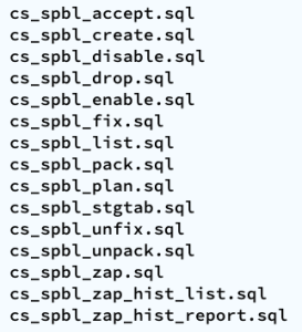
With the set of SQL Plan Baselines scripts, you can: 1) create a baseline based on a cursor or a plan stored into AWR; 2) enable and disable baselines; 3) drop baselines; 4) store them into a local staging table; 5) restore them from their local staging table; 6) promote as “fixed” or demote from “fixed”; 7) “zap” them if you have installed “El Zapper” (iod_spm).
Note: “El Zapper” is a PL/SQL package that extends the functionality of SQL Plan Management by automagically creating SQL Plan Baselines based on proven performance of a SQL statement over time, while considering a large number of executions, and a variety of historical plans. Please do not confuse “El Zapper” with auto-evolve of SPM. They are based on two very distinct premises. “El Zapper” also monitors the performance of active SQL Plan Baselines, and during an observation window it may disable a SQL Plan Baseline, if such plan no longer performs as “promised” (according to some thresholds). Most applications do not need “El Zapper”, since the use of SQL Plan Management should be more of an exception than a rule.
SQL Profiles scripts
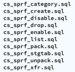
With the set of SQL Profiles scripts, you can: 1) create a profile based on the outline of a cursor, or from a plan stored into AWR; 2) enable and disable profiles; 3) drop profiles; 4) store them into a local staging table; 5) restore them from their local staging table; 6) transfer them from one location to another (very similar to coe_xfr_sql_profile.sql, but on a more modular way).
Note: Regarding the transfer of a SQL Profile, the concept is simple: 1) on source location generate two plain text scripts, one that contains the SQL text, and a second that includes the Execution Plan (outline); 2) execute these two scripts on a target location, in order to create a SQL Profile there. The beauty of this method is not only that you can easily move Execution Plans between locations, but that you can actually create a SQL Profile getting the SQL Text from SQL_ID “A”, and the Execution Plan from SQL_ID “B”, allowing you to do things like: removing CBO Hints, or using a plan from a similar SQL but not quite the same (e.g. I can tweak a stand-alone cloned version of a SQL statement, and once I get the plan that I need, I associate the SQL Text from the original SQL, with the desired Execution Plan out of the stand-alone customized version of the SQL, after that I create a SQL Plan Baseline and drop the staging SQL Profile).
SQL Patches scripts
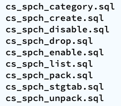
With the set of SQL Patches scripts, you can: 1) create a SQL patch based on one or more CBO Hints you provide (e.g.: GATHER_PLAN_STATISTICS MONITOR FIRST_ROWS(1) OPT_PARAM(‘_fix_control’ ‘5922070:OFF’) NO_BIND_AWARE); 2) enable and disable SQL patches; 3) drop SQL patches; 4) store them into a local staging table; 5) restore them from their local staging table.
Note: I use SQL Patches a lot, specially to embed CBO Hints that generate some desirable diagnostics details (and not so much to change plans), such as the ones provided by GATHER_PLAN_STATISTICS and MONITOR. In some cases, after I use the pathfinder tool written by Mauro Pagano, I have to disable a CBO patch (funny thing: I use a SQL Patch to disable a CBO Patch!). I also use a SQL Patch if I need to enable Adaptive Cursor Sharing (ACS) for one SQL (we disabled ACS for one major application). Bear in mind that SQL Plan Baselines, SQL Profiles and SQL Patches happily co-exist, so you can use them together, but I do prefer to use SQL Plan Baselines alone, whenever possible.
Introducing SQLdb360: merging eDB360 and SQLd360, while rising the bar to community engagement
Today, we are very happy to release SQLdb360, a new tool that merges together eDB360 and SQLd360, under a single package.
Tools eDB360 and SQLd360 can still be used independently, but now there is only one package to download and keep updated. All the new features and updates to both tools are now in that one package.
The biggest change that comes with SQLdb360 is the kind invitation to everyone interested to contribute to its development. This is why the new blended name and its release format.
We do encourage your help and ideas to continue building a free, open-source, and hopefully a YMMV great tool!
Over the years, a few community members requested new features, but they were ultimately slowed down by our speed of reaction to their requests. Well, no more!
Few consumers of these tools implemented cool changes they needed, sometimes sending us the changes (or pull requests) until a later time. This means good ideas were available to others after some time. Not anymore!
If there is something you’d like to have as part of SQLdb360 (aka SQLd360 and eDB360), just write and test the additional code, then send us the pull request! Next, we will review, validate, and merge your code changes to the main tool.
There are several advantages to this new approach:
- Carlos and Mauro won’t dictate the direction of the tool anymore: we will continue helping and contributing, but we won’t “own” it anymore (the community will!)
- Carlos and Mauro won’t slow down the development anymore: nobody is the bottleneck now!
- Carlos and Mauro wan’t run out of ideas anymore!!! The community has great ideas to share!!!
Due to the nature of this new collaborative effort, the way we now publish SQLdb360 is this:
- Instead of linking to the current master repository, the tool now implements “releases”. This, in order to snapshot stable versions that bundle several changes together (better than creating separate versions per merge into master).
- Links in our blogs are now getting updated, with references to the latest (and current) stable release of SQLdb360 (starting with v18.1).
Note: Version names sound awfully familiar to Oracle nomenclature, right? Well, we started using this numbering back in 2014!!!
Carlos & Mauro
Adapting and adopting SQL Plan Management (SPM)
Introduction
This post is about: “Adapting and adopting SQL Plan Management (SPM) to achieve execution plan stability for sub-second queries on a high-rate OLTP mission-critical application”. In our case, such an application is implemented on top of several Oracle 12c multi tenant databases, where a consistent average execution time is more valuable than flexible execution plans. We successfully achieved plan stability implementing a simple algorithm using PL/SQL calling DBMS_SPM public APIs.
Chart below depicts a typical case where the average performance of a large set of business-critical SQL statements suddenly degraded from sub-millisecond to 15 or 20ms, then beccome more stable around 3ms. Wide spikes are a typical trademark of an Execution Plan for one or more SQL statements flipping for some time. In order to produce a more consistent latency we needed to improve plan stability, and of course the preferred tool to achieve that on an Oracle database is SQL Plan Management.

Algorithm
We tested and ruled out adaptive SQL Plan Management, which is an excellent 12c new feature. But, due to the dynamics of this application, where transactional data shifts so fast, allowing this “adaptive SPM” feature to evaluate auto-captured plans using bind variable values captured a few hours earlier, rendered unfortunately false positives. These false positives “evolved” as execution plans that were numerically optimal for values captured (at the time the candidate plan was captured), but performed poorly when executed on “current” values a few hours later. Nevertheless, this 12c “adaptive SPM” new feature is worth exploring for other applications.
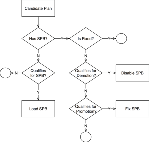 We adapted SPM so it would only generate SQL Plan Baselines on SQL that executes often, and that is critical for the business. The algorithm has some complexity such as candidate evaluation and SQL categorization; and besides SPB creation it also includes plan demotion and plan promotion. We have successfully implemented it in some PDBs and we are currently doing a rollout to entire CDBs. The algorithm is depicted on diagram on the left, and more details are included in corresponding presentation slides listed on the right-hand bar. I plan to talk about this topic on an international Oracle Users Group in 2018.
This algorithm is scripted into a sample PL/SQL package, which you can find on a subdirectory on my shared scripts. If you consider using this sample script for an application of your own, be sure you make it yours before attempting to use it. In other words: fully understand it first, then proceed to customize it accordingly and test it thoroughly.
Results
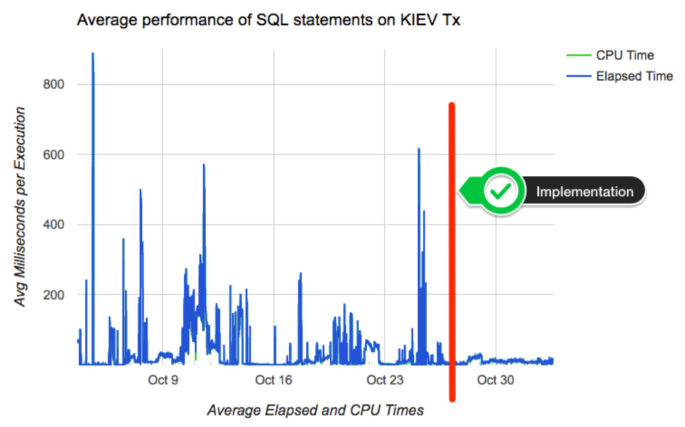
Chart below shows how average performance of business-critical SQL became more stable after implementing algorithm to adapt and adopt SPM on a pilot PDB. Not all went fine although: we had some outliers that required some tuning to the algorithm. Among challenges we faced: volatile data (creating a SPB when table was almost empty, then using it when table was larger); skewed values (create a SPB for non-popular value, then using it on a popular value); proper use of multiple optimal plans due to Adaptive Cursor Sharing (ACS); rejected candidates due to conservative initial restrictions on algorithm (performance per execution, number of executions, age of cursor, etc.)
Conclusion
If your OLTP application contains business critical SQL that executes at a high-rate, and where a spike on latency risks affecting SLAs, you may want to consider implementing SQL Plan Management. Consider then both: “adaptive SPM” if it satisfies your requirements, else build a PL/SQL library that can implement more complex logic for candidates evaluation and for SPBs maintenance. I do believe SPM works great, specially when you enhance its out-of-the-box functionality to satisfy your specific needs.
Creating a SQL Plan Baseline from Cursor Cache or AWR
A DBA deals with performance issues often, and having a SQL suddenly performing poorly is common. What do we do? We proceed to “pin” an execution plan, then investigate root cause (the latter is true if time to next fire permits).
DBMS_SPM provides some APIs to create a SQL Plan Baseline (SPB) from the Cursor Cache, or from a SQL Tuning Set (STS), but not from the Automatic Workload Repository (AWR). For the latter, you need a two-steps approach: create a STS from AWR, then load a SPB from the STS. Fine, except when your next fire is waiting for you, or when deciding which is the “best” plan is not trivial.
Take for example chart below, which depicts multiple execution plans with different performance for one SQL statement. The SQL statement is actually quite simple, and data is not significantly skewed. On this particular application, usually one-size-fits-all (meaning one-and-only-one plan) works well for most values passed on variable place holders. Then, which plan would you choose?

Note: please get all scripts using the download column on the right
Looking at summary of known Execution Plans’ performance below (as reported by planx.sql), we can see the same 6 Execution Plans.
1st Plan on list shows an average execution time of 2.897ms according to AWR, and 0.896ms according to Cursor Cache; and number of recorded executions for this Plan are 2,502 and 2,178 respectively. We see this Plan contains one Nested Loop, and if we look at historical performance we notice this Plan takes less than 109ms 95% of the time, less than 115ms 97% of the time, and less then 134ms 99% of the time. We also see that worst recorded AWR period, had this SQL performing in under 150ms (on average for that one period).
We also notice that last plan on list performs one execution in 120.847ms on average (as per AWR) and 181.113ms according to Cursor Cache (on average as well). Then, “pinning” 1st plan on list seems like a good choice, but not too different than all but last plan, specially when we consider both: average performance and historical performance according to percentiles reported.
PLANS PERFORMANCE
~~~~~~~~~~~~~~~~~

       Plan ET Avg      ET Avg      CPU Avg     CPU Avg           BG Avg       BG Avg   Executions   Executions                                   ET 100th    ET 99th     ET 97th     ET 95th     CPU 100th   CPU 99th    CPU 97th    CPU 95th
 Hash Value AWR (ms)    MEM (ms)    AWR (ms)    MEM (ms)             AWR          MEM          AWR          MEM   MIN Cost   MAX Cost  NL  HJ  MJ Pctl (ms)   Pctl (ms)   Pctl (ms)   Pctl (ms)   Pctl (ms)   Pctl (ms)   Pctl (ms)   Pctl (ms)
----------- ----------- ----------- ----------- ----------- ------------ ------------ ------------ ------------ ---------- ---------- --- --- --- ----------- ----------- ----------- ----------- ----------- ----------- ----------- -----------
 4113179674       2.897       0.896       2.715       0.714           96            5        2,502        2,178          8        738   1   0   0     149.841     133.135     114.305     108.411     147.809     133.007     113.042     107.390
  578709260      29.576      32.704      28.865      31.685        1,583        1,436        6,150        1,843         67        875   1   0   0     154.560      84.264      65.409      57.311     148.648      75.209      62.957      56.305
 1990606009      74.399      79.054      73.163      77.186        1,117        1,192          172          214        905      1,108   0   1   0     208.648     208.648      95.877      95.351     205.768     205.768      94.117      93.814
 1242077371      77.961                  77.182                    1,772                     8,780                     949      1,040   0   1   0     102.966      98.206      91.163      89.272     100.147      97.239      90.165      88.412
 2214147219      79.650      82.413      78.242      80.817        1,999        2,143       42,360       24,862        906      1,242   0   1   0     122.535     101.293      98.442      95.737     119.240      99.118      95.266      93.156
 1214505235     120.847     181.113     105.485     162.783          506        1,355           48           12        114        718   1   0   0     285.950     285.950     285.950     285.950     193.954     193.954     193.954     193.954
Plans performance summary above is displayed in a matter of seconds by planx.sql, sqlperf.sql and by a new script spb_create.sql. This output helps make a quick decision about which Execution Plan is better for “pinning”, meaning: to create a SPB on it.
Sometimes such decision is not that trivial, as we can see on sample below. Which plan is better? I would go with 2nd on list. Why? performance-wise this plan is more stable. It does a Hash Join, so I am expecting to see a Plan with full scans, but if I can get consistent executions under 0.4s (according to percentiles), I would be tempted to “pin” this 2nd Plan instead of 1st one. And I would stay away from 3rd and 5th. So maybe I would create a SPB with 3 plans instead of just one, and include on this SPB 1st, 2nd and 4th on the list.
PLANS PERFORMANCE
~~~~~~~~~~~~~~~~~

       Plan ET Avg      ET Avg      CPU Avg     CPU Avg           BG Avg       BG Avg   Executions   Executions                                   ET 100th    ET 99th     ET 97th     ET 95th     CPU 100th   CPU 99th    CPU 97th    CPU 95th
 Hash Value AWR (ms)    MEM (ms)    AWR (ms)    MEM (ms)             AWR          MEM          AWR          MEM   MIN Cost   MAX Cost  NL  HJ  MJ Pctl (ms)   Pctl (ms)   Pctl (ms)   Pctl (ms)   Pctl (ms)   Pctl (ms)   Pctl (ms)   Pctl (ms)
----------- ----------- ----------- ----------- ----------- ------------ ------------ ------------ ------------ ---------- ---------- --- --- --- ----------- ----------- ----------- ----------- ----------- ----------- ----------- -----------
 1917891576       0.467       0.334       0.330       0.172          119           33  554,914,504   57,748,249          6      1,188   2   0   0   6,732.017      10.592       1.628       1.572   1,420.864       1.557       1.482       1.261
   99953997       1.162       2.427       0.655       0.492           83           55   58,890,160    2,225,247         12      2,311   0   1   0     395.819     235.474     108.142      34.909      56.008      22.329      12.926       3.069
 3559532534       1.175   1,741.041       0.858      91.486          359           46   21,739,877          392          4         20   1   0   0  89,523.768   4,014.301     554.740     298.545  21,635.611     216.456      54.050      30.130
 3650324870       2.028      20.788       1.409       2.257          251          199   24,038,404      143,819         11      5,417   0   1   0     726.964     254.245      75.322      20.817     113.259      21.211      13.591       8.486
 3019880278      43.465                  43.029                   20,217                    13,349                   5,693      5,693   0   1   0      43.465      43.465      43.465      43.465      43.029      43.029      43.029      43.029
About new script spb_create.sql
Update: Scripts to deal with SQL Plan Baselines, SQL Profiles and SQL Patches
This new script is a life-saver for us, since our response time for an alert is usually measured in minutes, with a resolution (and sometimes a root cause analysis) expected in less than one hour from the time the incident is raised.
This script is quite simple:
- it provides a list of known Execution Plans including current (Cursor Cache) and historical (AWR) performance as displayed in two samples above, then
- asks on which Plan Hash Values (PHVs) you want to create a SPB on. It allows you to enter up to 3 PHVs; last
- asks if you want these plans to be set as FIXED
After you respond to ACCEPT parameters, then a SPB for your SQL is created and displayed. It does not matter if the Plan exists on Cursor Cache and/or on AWR, it finds the Plan and creates the SPB for you. Then: finding known Execution Plans, deciding which one is a better choice (or maybe more than one), and creating a SPB, all can be done very rapidly.
If you still prefer to use SQL Profiles and not SPBs for whatever reason, script coe_xfr_sql_profile.sql is still around and updated. On these 12c days, and soon 18c and beyond, I’d much rather use SQL Plan Management and create SPBs although!
Anyways, enjoy these free scripts and become a faster hero “pinning” good plans. Then don’t forget to do diligent root cause analysis afterwards. I use SQLd360 by Mauro Pagano for deep understanding of what is going on with my SQL statements.
Soon, I will post about a cool free tool that automates the implementation of SQL Plan Management on a high-rate OLTP where stability is more important than flexibility (frequently changing Execution Plans). Stay tuned!
Note: please get all scripts using the download column on the right
Purging a cursor in Oracle – revisited
A few years ago I created a post about “how to flush a cursor out the shared pool“, using DBMS_SHARED_POOL.PURGE. For the most part, this method has helped me to get rid of an entire parent cursor and all child cursors for a given SQL, but more often than not I have found than on 12c this method may not work, leaving active a set of cursors I want to flush.
Script below is an enhanced version, where besides using DBMS_SHARED_POOL.PURGE, we also create a dummy SQL patch, then drop it. This method seems to completely flush parent and child cursors. Why using this method instead?: We are implementing SQL Plan Management (SPM), and we have found that in some cases, some child cursors are still shared several hours after a SQL Plan Baseline (SPB) is created. We could argue a possible bug and pursue as such, but in the meantime my quick and dirty workaround is: whenever I want to flush an individual parent cursor for one SQL, and all of its child cursors, I just execute script below passing SQL_ID.
Anyways, just wanted to share and document this purge_cursor.sql script for those in similar need. I have developed it on 12.1.0.2, and haven’t tested it on lower or higher versions.
-- purge_cursor.sql
DECLARE
 l_name VARCHAR2(64);
 l_sql_text CLOB;
BEGIN
 -- get address, hash_value and sql text
 SELECT address||','||hash_value, sql_fulltext
 INTO l_name, l_sql_text
 FROM v$sqlarea
 WHERE sql_id = '&&sql_id.';
 -- not always does the job
 SYS.DBMS_SHARED_POOL.PURGE (
 name => l_name,
 flag => 'C',
 heaps => 1
 );
 -- create fake sql patch
 SYS.DBMS_SQLDIAG_INTERNAL.I_CREATE_PATCH (
 sql_text => l_sql_text,
 hint_text => 'NULL',
 name => 'purge_&&sql_id.',
 description => 'PURGE CURSOR',
 category => 'DEFAULT',
 validate => TRUE
 );
 -- drop fake sql patch
 SYS.DBMS_SQLDIAG.DROP_SQL_PATCH (
 name => 'purge_&&sql_id.',
 ignore => TRUE
 );
END;
/
