Archive for the ‘AWR’ Category
Scripts to deal with SQL Plan Baselines, SQL Profiles and SQL Patches
To mitigate SQL performance issues, I do make use of SQL Plan Baselines, SQL Profiles and SQL Patches, on a daily basis. Our environments are single-instance 12.1.0.2 CDBs, with over 2,000 PDBs. Our goal is Execution Plan Stability and consistent performance, over CBO plan flexibility. The CBO does a good job, considering the complexity imposed by current applications design. Nevertheless, some SQL require some help in order to enhance their plan stability.
I have written and shared a set of scripts that simply make the use of a bunch of APIs a lot easier, with better documented actions, and fully consistent within the organization. I have shared with the community these scripts in the past, and I keep them updated as per needs change. All these “CS” scripts are available under the download section on the right column.
Current version of the CS scripts is more like a toolset. You treat them as a whole. All of them call some other script that exists within the cs_internal subdirectory, then I usually navigate to the parent sql directory, and connect into SQL*Plus from there. All these scripts can be easily cloned and/or customized to your specific needs. They are available as “free to use” and “as is”. There is no requirement to keep their heading intact, so you can reverse-engineer them and make them your own if you want. Just keep in mind that I maintain, enhance, and extend this CS toolset every single day; so what you get today is a subset of what you will get tomorrow. If you think an enhancement you need (or a fix) is beneficial to the larger community (and to you), please let me know.
SQL Plan Baselines scripts

With the set of SQL Plan Baselines scripts, you can: 1) create a baseline based on a cursor or a plan stored into AWR; 2) enable and disable baselines; 3) drop baselines; 4) store them into a local staging table; 5) restore them from their local staging table; 6) promote as “fixed” or demote from “fixed”; 7) “zap” them if you have installed “El Zapper” (iod_spm).
Note: “El Zapper” is a PL/SQL package that extends the functionality of SQL Plan Management by automagically creating SQL Plan Baselines based on proven performance of a SQL statement over time, while considering a large number of executions, and a variety of historical plans. Please do not confuse “El Zapper” with auto-evolve of SPM. They are based on two very distinct premises. “El Zapper” also monitors the performance of active SQL Plan Baselines, and during an observation window it may disable a SQL Plan Baseline, if such plan no longer performs as “promised” (according to some thresholds). Most applications do not need “El Zapper”, since the use of SQL Plan Management should be more of an exception than a rule.
SQL Profiles scripts
With the set of SQL Profiles scripts, you can: 1) create a profile based on the outline of a cursor, or from a plan stored into AWR; 2) enable and disable profiles; 3) drop profiles; 4) store them into a local staging table; 5) restore them from their local staging table; 6) transfer them from one location to another (very similar to coe_xfr_sql_profile.sql, but on a more modular way).
Note: Regarding the transfer of a SQL Profile, the concept is simple: 1) on source location generate two plain text scripts, one that contains the SQL text, and a second that includes the Execution Plan (outline); 2) execute these two scripts on a target location, in order to create a SQL Profile there. The beauty of this method is not only that you can easily move Execution Plans between locations, but that you can actually create a SQL Profile getting the SQL Text from SQL_ID “A”, and the Execution Plan from SQL_ID “B”, allowing you to do things like: removing CBO Hints, or using a plan from a similar SQL but not quite the same (e.g. I can tweak a stand-alone cloned version of a SQL statement, and once I get the plan that I need, I associate the SQL Text from the original SQL, with the desired Execution Plan out of the stand-alone customized version of the SQL, after that I create a SQL Plan Baseline and drop the staging SQL Profile).
SQL Patches scripts
With the set of SQL Patches scripts, you can: 1) create a SQL patch based on one or more CBO Hints you provide (e.g.: GATHER_PLAN_STATISTICS MONITOR FIRST_ROWS(1) OPT_PARAM(‘_fix_control’ ‘5922070:OFF’) NO_BIND_AWARE); 2) enable and disable SQL patches; 3) drop SQL patches; 4) store them into a local staging table; 5) restore them from their local staging table.
Note: I use SQL Patches a lot, specially to embed CBO Hints that generate some desirable diagnostics details (and not so much to change plans), such as the ones provided by GATHER_PLAN_STATISTICS and MONITOR. In some cases, after I use the pathfinder tool written by Mauro Pagano, I have to disable a CBO patch (funny thing: I use a SQL Patch to disable a CBO Patch!). I also use a SQL Patch if I need to enable Adaptive Cursor Sharing (ACS) for one SQL (we disabled ACS for one major application). Bear in mind that SQL Plan Baselines, SQL Profiles and SQL Patches happily co-exist, so you can use them together, but I do prefer to use SQL Plan Baselines alone, whenever possible.
Creating a SQL Plan Baseline from Cursor Cache or AWR
A DBA deals with performance issues often, and having a SQL suddenly performing poorly is common. What do we do? We proceed to “pin” an execution plan, then investigate root cause (the latter is true if time to next fire permits).
DBMS_SPM provides some APIs to create a SQL Plan Baseline (SPB) from the Cursor Cache, or from a SQL Tuning Set (STS), but not from the Automatic Workload Repository (AWR). For the latter, you need a two-steps approach: create a STS from AWR, then load a SPB from the STS. Fine, except when your next fire is waiting for you, or when deciding which is the “best” plan is not trivial.
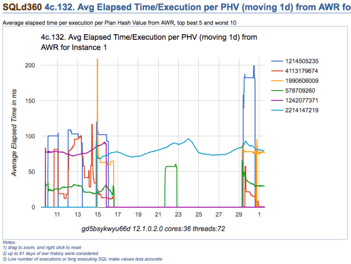
Take for example chart below, which depicts multiple execution plans with different performance for one SQL statement. The SQL statement is actually quite simple, and data is not significantly skewed. On this particular application, usually one-size-fits-all (meaning one-and-only-one plan) works well for most values passed on variable place holders. Then, which plan would you choose?
Note: please get all scripts using the download column on the right
Looking at summary of known Execution Plans’ performance below (as reported by planx.sql), we can see the same 6 Execution Plans.
1st Plan on list shows an average execution time of 2.897ms according to AWR, and 0.896ms according to Cursor Cache; and number of recorded executions for this Plan are 2,502 and 2,178 respectively. We see this Plan contains one Nested Loop, and if we look at historical performance we notice this Plan takes less than 109ms 95% of the time, less than 115ms 97% of the time, and less then 134ms 99% of the time. We also see that worst recorded AWR period, had this SQL performing in under 150ms (on average for that one period).
We also notice that last plan on list performs one execution in 120.847ms on average (as per AWR) and 181.113ms according to Cursor Cache (on average as well). Then, “pinning” 1st plan on list seems like a good choice, but not too different than all but last plan, specially when we consider both: average performance and historical performance according to percentiles reported.
PLANS PERFORMANCE
~~~~~~~~~~~~~~~~~

       Plan ET Avg      ET Avg      CPU Avg     CPU Avg           BG Avg       BG Avg   Executions   Executions                                   ET 100th    ET 99th     ET 97th     ET 95th     CPU 100th   CPU 99th    CPU 97th    CPU 95th
 Hash Value AWR (ms)    MEM (ms)    AWR (ms)    MEM (ms)             AWR          MEM          AWR          MEM   MIN Cost   MAX Cost  NL  HJ  MJ Pctl (ms)   Pctl (ms)   Pctl (ms)   Pctl (ms)   Pctl (ms)   Pctl (ms)   Pctl (ms)   Pctl (ms)
----------- ----------- ----------- ----------- ----------- ------------ ------------ ------------ ------------ ---------- ---------- --- --- --- ----------- ----------- ----------- ----------- ----------- ----------- ----------- -----------
 4113179674       2.897       0.896       2.715       0.714           96            5        2,502        2,178          8        738   1   0   0     149.841     133.135     114.305     108.411     147.809     133.007     113.042     107.390
  578709260      29.576      32.704      28.865      31.685        1,583        1,436        6,150        1,843         67        875   1   0   0     154.560      84.264      65.409      57.311     148.648      75.209      62.957      56.305
 1990606009      74.399      79.054      73.163      77.186        1,117        1,192          172          214        905      1,108   0   1   0     208.648     208.648      95.877      95.351     205.768     205.768      94.117      93.814
 1242077371      77.961                  77.182                    1,772                     8,780                     949      1,040   0   1   0     102.966      98.206      91.163      89.272     100.147      97.239      90.165      88.412
 2214147219      79.650      82.413      78.242      80.817        1,999        2,143       42,360       24,862        906      1,242   0   1   0     122.535     101.293      98.442      95.737     119.240      99.118      95.266      93.156
 1214505235     120.847     181.113     105.485     162.783          506        1,355           48           12        114        718   1   0   0     285.950     285.950     285.950     285.950     193.954     193.954     193.954     193.954
Plans performance summary above is displayed in a matter of seconds by planx.sql, sqlperf.sql and by a new script spb_create.sql. This output helps make a quick decision about which Execution Plan is better for “pinning”, meaning: to create a SPB on it.
Sometimes such decision is not that trivial, as we can see on sample below. Which plan is better? I would go with 2nd on list. Why? performance-wise this plan is more stable. It does a Hash Join, so I am expecting to see a Plan with full scans, but if I can get consistent executions under 0.4s (according to percentiles), I would be tempted to “pin” this 2nd Plan instead of 1st one. And I would stay away from 3rd and 5th. So maybe I would create a SPB with 3 plans instead of just one, and include on this SPB 1st, 2nd and 4th on the list.
PLANS PERFORMANCE
~~~~~~~~~~~~~~~~~

       Plan ET Avg      ET Avg      CPU Avg     CPU Avg           BG Avg       BG Avg   Executions   Executions                                   ET 100th    ET 99th     ET 97th     ET 95th     CPU 100th   CPU 99th    CPU 97th    CPU 95th
 Hash Value AWR (ms)    MEM (ms)    AWR (ms)    MEM (ms)             AWR          MEM          AWR          MEM   MIN Cost   MAX Cost  NL  HJ  MJ Pctl (ms)   Pctl (ms)   Pctl (ms)   Pctl (ms)   Pctl (ms)   Pctl (ms)   Pctl (ms)   Pctl (ms)
----------- ----------- ----------- ----------- ----------- ------------ ------------ ------------ ------------ ---------- ---------- --- --- --- ----------- ----------- ----------- ----------- ----------- ----------- ----------- -----------
 1917891576       0.467       0.334       0.330       0.172          119           33  554,914,504   57,748,249          6      1,188   2   0   0   6,732.017      10.592       1.628       1.572   1,420.864       1.557       1.482       1.261
   99953997       1.162       2.427       0.655       0.492           83           55   58,890,160    2,225,247         12      2,311   0   1   0     395.819     235.474     108.142      34.909      56.008      22.329      12.926       3.069
 3559532534       1.175   1,741.041       0.858      91.486          359           46   21,739,877          392          4         20   1   0   0  89,523.768   4,014.301     554.740     298.545  21,635.611     216.456      54.050      30.130
 3650324870       2.028      20.788       1.409       2.257          251          199   24,038,404      143,819         11      5,417   0   1   0     726.964     254.245      75.322      20.817     113.259      21.211      13.591       8.486
 3019880278      43.465                  43.029                   20,217                    13,349                   5,693      5,693   0   1   0      43.465      43.465      43.465      43.465      43.029      43.029      43.029      43.029
About new script spb_create.sql
Update: Scripts to deal with SQL Plan Baselines, SQL Profiles and SQL Patches
This new script is a life-saver for us, since our response time for an alert is usually measured in minutes, with a resolution (and sometimes a root cause analysis) expected in less than one hour from the time the incident is raised.
This script is quite simple:
- it provides a list of known Execution Plans including current (Cursor Cache) and historical (AWR) performance as displayed in two samples above, then
- asks on which Plan Hash Values (PHVs) you want to create a SPB on. It allows you to enter up to 3 PHVs; last
- asks if you want these plans to be set as FIXED
After you respond to ACCEPT parameters, then a SPB for your SQL is created and displayed. It does not matter if the Plan exists on Cursor Cache and/or on AWR, it finds the Plan and creates the SPB for you. Then: finding known Execution Plans, deciding which one is a better choice (or maybe more than one), and creating a SPB, all can be done very rapidly.
If you still prefer to use SQL Profiles and not SPBs for whatever reason, script coe_xfr_sql_profile.sql is still around and updated. On these 12c days, and soon 18c and beyond, I’d much rather use SQL Plan Management and create SPBs although!
Anyways, enjoy these free scripts and become a faster hero “pinning” good plans. Then don’t forget to do diligent root cause analysis afterwards. I use SQLd360 by Mauro Pagano for deep understanding of what is going on with my SQL statements.
Soon, I will post about a cool free tool that automates the implementation of SQL Plan Management on a high-rate OLTP where stability is more important than flexibility (frequently changing Execution Plans). Stay tuned!
Note: please get all scripts using the download column on the right
eDB360 meets eAdam 3.0 – when two heads are better than one!

Version v1711 of eDB360 invites eAdam 3.0 to the party. What does it mean? We recently learned that eDB360 v1706 introduced the eDB360 repository, which materialized the content of 26 core DBA_HIST views into a staging repository made of heap tables. This in order to expedite the execution of eDB360 on a database with an enlarged AWR. New version v1711 expands the list from 26 views to a total of 219. And these 219 views include now DBA_HIST, DBA, GV$ and V$.
Expanding existing eDB360 repository 8.4x from 26 to 219 views is not what is key on version v1710. The real impact of the latest version of eDB360 is that now it benefits of eAdam 3.0, providing the same benefits of the 219 views of the eDB360 heap-tables repository, but using External Tables, which are easily transported from a source database to a target database. This simple fact opens many doors.
Using the eAdam 3.0 repository from eDB360, we can now extract the metadata from a production database, then restore it on a staging database where we can produce the eDB360 report for the source database. We could also use this new external repository for: finer-granularity data mining; capacity planning; sizing for potential hardware refresh; provisioning tools; to estimate candidate segments for partitioning or for offloading into Hadoop; etc.
With the new external-tables eAdam 3.0 repository, we could easily build a permanent larger heap-table permanent repository for multiple databases (multiple tenants), or for multiple time versions of the same database. Thus, now that eDB360 has met eAdam 3.0, the combination of these two enables multiple innovative future features (custom or to be packaged and shipped with eDB360).
eDB360 recap
eDB360 is a free tool that gives a 360-degree view of an Oracle database. It installs nothing on the database, and it runs on 10g to 12c Oracle databases. It is designed for Linux and UNIX, but runs well on Windows as well (you may want to install first UNIX Utilities UnxUtils and a zip program, else a few OS commands may not properly work on Windows). This repository-less version is the default way to use eDB360, and is the right method for most cases. But now, in addition to the default use, eDB360 can also make use of one of two repositories.
eDB360 takes time to execute (several hours). It is designed to time-out after 24 hours by default. First reason for long execution times is the intentional serial-processing method used, with sequential execution of query after query, while consuming little resources. Such serial execution, plus the fact that it is common to have the tool execute on large databases where the state of AWR is suboptimal, causes the execution to take long. We often discover that source AWR repositories lack expected partitioning, and in many cases they hold years of data instead of expected 8 to 31 days. Therefore, the nature of serial-execution combined with enlarged and suboptimal AWR repositories, usually cause eDB360 to execute for many hours more than expected. With 8 to 31 days of AWR data, and when such reasonable history is well partitioned, eDB360 usually executes in less than 6 hours.
To overcome the undesired extended execution times of eDB360, and besides the obvious (partition and purge AWR), the tool provides the capability to execute in multiple threads splitting its content by column. And now, in addition to the divide-and-conquer approach of column execution, eDB360 provides 2 repositories with different objectives in mind:
- eDB360 repository: Use this method to create a staging repository based on heap tables inside the source database. This method helps to expedite the execution of eDB360 by at least 10x. Repository heap-tables are created and consumed inside the same database.
- eAdam3 repository: Use this method to generate a repository based on external tables on the source database. Such external-tables repository can be moved easily to a remote target system, allowing to efficiently generate the eDB360 report there. This method helps to reduce computations in the source database, and enables potential data mining on the external repository without any resources impact on the source database. This method also helps to build other functions on top of the 219-tables repository.
Views included on both eDB360 and eAdam3 repositories:
- dba_2pc_neighbors
- dba_2pc_pending
- dba_all_tables
- dba_audit_mgmt_config_params
- dba_autotask_client
- dba_autotask_client_history
- dba_cons_columns
- dba_constraints
- dba_data_files
- dba_db_links
- dba_extents
- dba_external_tables
- dba_feature_usage_statistics
- dba_free_space
- dba_high_water_mark_statistics
- dba_hist_active_sess_history
- dba_hist_database_instance
- dba_hist_event_histogram
- dba_hist_ic_client_stats
- dba_hist_ic_device_stats
- dba_hist_interconnect_pings
- dba_hist_memory_resize_ops
- dba_hist_memory_target_advice
- dba_hist_osstat
- dba_hist_parameter
- dba_hist_pgastat
- dba_hist_resource_limit
- dba_hist_seg_stat
- dba_hist_service_name
- dba_hist_sga
- dba_hist_sgastat
- dba_hist_snapshot
- dba_hist_sql_plan
- dba_hist_sqlstat
- dba_hist_sqltext
- dba_hist_sys_time_model
- dba_hist_sysmetric_history
- dba_hist_sysmetric_summary
- dba_hist_sysstat
- dba_hist_system_event
- dba_hist_tbspc_space_usage
- dba_hist_wr_control
- dba_ind_columns
- dba_ind_partitions
- dba_ind_statistics
- dba_ind_subpartitions
- dba_indexes
- dba_jobs
- dba_jobs_running
- dba_lob_partitions
- dba_lob_subpartitions
- dba_lobs
- dba_obj_audit_opts
- dba_objects
- dba_pdbs
- dba_priv_audit_opts
- dba_procedures
- dba_profiles
- dba_recyclebin
- dba_registry
- dba_registry_hierarchy
- dba_registry_history
- dba_registry_sqlpatch
- dba_role_privs
- dba_roles
- dba_rsrc_consumer_group_privs
- dba_rsrc_consumer_groups
- dba_rsrc_group_mappings
- dba_rsrc_io_calibrate
- dba_rsrc_mapping_priority
- dba_rsrc_plan_directives
- dba_rsrc_plans
- dba_scheduler_job_log
- dba_scheduler_jobs
- dba_scheduler_windows
- dba_scheduler_wingroup_members
- dba_segments
- dba_sequences
- dba_source
- dba_sql_patches
- dba_sql_plan_baselines
- dba_sql_plan_dir_objects
- dba_sql_plan_directives
- dba_sql_profiles
- dba_stat_extensions
- dba_stmt_audit_opts
- dba_synonyms
- dba_sys_privs
- dba_tab_cols
- dba_tab_columns
- dba_tab_modifications
- dba_tab_partitions
- dba_tab_privs
- dba_tab_statistics
- dba_tab_subpartitions
- dba_tables
- dba_tablespace_groups
- dba_tablespaces
- dba_temp_files
- dba_triggers
- dba_ts_quotas
- dba_unused_col_tabs
- dba_users
- dba_views
- gv$active_session_history
- gv$archive_dest
- gv$archived_log
- gv$asm_disk_iostat
- gv$database
- gv$dataguard_status
- gv$event_name
- gv$eventmetric
- gv$instance
- gv$instance_recovery
- gv$latch
- gv$license
- gv$managed_standby
- gv$memory_current_resize_ops
- gv$memory_dynamic_components
- gv$memory_resize_ops
- gv$memory_target_advice
- gv$open_cursor
- gv$osstat
- gv$parameter
- gv$pga_target_advice
- gv$pgastat
- gv$pq_slave
- gv$pq_sysstat
- gv$process
- gv$process_memory
- gv$px_buffer_advice
- gv$px_process
- gv$px_process_sysstat
- gv$px_session
- gv$px_sesstat
- gv$resource_limit
- gv$result_cache_memory
- gv$result_cache_statistics
- gv$rsrc_cons_group_history
- gv$rsrc_consumer_group
- gv$rsrc_plan
- gv$rsrc_plan_history
- gv$rsrc_session_info
- gv$rsrcmgrmetric
- gv$rsrcmgrmetric_history
- gv$segstat
- gv$services
- gv$session
- gv$session_blockers
- gv$session_wait
- gv$sga
- gv$sga_target_advice
- gv$sgainfo
- gv$sgastat
- gv$sql
- gv$sql_monitor
- gv$sql_plan
- gv$sql_shared_cursor
- gv$sql_workarea_histogram
- gv$sysmetric
- gv$sysmetric_summary
- gv$sysstat
- gv$system_parameter2
- gv$system_wait_class
- gv$temp_extent_pool
- gv$undostat
- gv$waitclassmetric
- gv$waitstat
- v$archive_dest_status
- v$archived_log
- v$ash_info
- v$asm_attribute
- v$asm_client
- v$asm_disk
- v$asm_disk_stat
- v$asm_diskgroup
- v$asm_diskgroup_stat
- v$asm_file
- v$asm_template
- v$backup
- v$backup_set_details
- v$block_change_tracking
- v$cell_config
- v$cell_state
- v$controlfile
- v$database
- v$database_block_corruption
- v$datafile
- v$flashback_database_log
- v$flashback_database_stat
- v$instance
- v$io_outlier
- v$iostat_file
- v$kernel_io_outlier
- v$lgwrio_outlier
- v$log
- v$log_history
- v$logfile
- v$mystat
- v$nonlogged_block
- v$option
- v$parallel_degree_limit_mth
- v$parameter
- v$pdbs
- v$recovery_area_usage
- v$recovery_file_dest
- v$restore_point
- v$rman_backup_job_details
- v$rman_output
- v$segstat
- v$spparameter
- v$standby_log
- v$sys_time_model
- v$sysaux_occupants
- v$system_parameter2
- v$tablespace
- v$tempfile
- v$thread
- v$version
Instructions to use eDB360 and eAdam3 repositories
Both repositories are implemented under the edb360-master/repo subdirectory. Each has a readme file, which explains how to create the repository, consume it and drop it. The eAdam3 repository also includes instructions how to clone an external-table-based eAdam repository into a heap-table-based eDB360 repository.
Executing eDB360 on the eDB360 repository is faster than executing it on the eAdam3 repository, while avoiding new bug 25802477. This new Oracle database bug inflicts compressed external-tables like the ones used by the eAdam3 repository.
If you use eDB360 or eAdam3 repositories and have questions or concerns, do not hesitate to contact the author.
eDB360 new features (March 2017)

As many of you know, eDB360 is a free tool that provides a 360-degree view of an Oracle database without any installation. A new version is available like once per month, but occasionally a large number of enhancements are implemented at once. This new release v1708 (March 25, 2017) includes several new features requested recently by some users of the tool, thus the need to blog about what is new:
- Reducing the scope of eDB360 is now possible without having to generate a custom configuration file. Prior to this version, if a user wanted to generate output for let’s say AWR reports only (section 7a), the tool needed a custom.sql file with line DEF edb360_sections = ‘7a’;. Then we would pass to edb360.sql as 2nd execution parameter the name of this custom configuration file (too cumbersome!). Starting on v1708, we can directly pass to edb360.sql the section that we desire (i.e. SQL> @edb360 T 7a). This 2nd parameter can either input the name of a custom configuration file (legacy functionality), but now it also accepts a column, a section, a list of columns or a list of sections; for example: 7a, 7, 7a-7b, 1-4 and 3 are all valid values.
- A couple of reports were added to section 3h: “SQL in logon storms” and “SQL executed row-by-row”. The former identifies those SQL statements that are seen frequently on very short-lived sessions (based on ASH), and the latter presents a list of SQL statements with large number of executions and small number of rows processed.
- eDB360 now extracts ASH from eAdam for top 16 SQL_ID (as per SQLd360 list) + top 12 SNAP_ID (as per AWR MAX from column 7a). What it means is that eDB360 includes now a tar file with raw ASH data for both: SQL statements of interest and for AWR periods of interest (both according to what eDB360 considers important). Using eAdam is easy, so when content of eDB360 does not include a very specific aggregation of ASH data that we need, or when we have to understand the sequence of some ASH samples for example, we can then restore this eAdam data on any Oracle database and data mine it.
- Some reports on section 2b show now totals at the bottom. That is to SUM some numeric values. Other reports may follow in future releases.
- RMAN section includes now a new report “Blocks with Corruption or Non-logged”.
- Added Load Profile (Per Sec, Per Txn and Count) as per DBA_HIST_SYSMETRIC_SUMMARY. This Load Profile resembles what we see on AWR at the top, but this is computed for the entire period of diagnostics (31 days by default). It shows max values, average, median and several percentiles. With this new report on section 1a, we can glance over it and discover in minutes some areas of further interest, for example: logons per second too high, just to mention one.
- There is a new section 4i with “Waits Count v.s. Average Latency for top 24 Wait Events”. With this set of 24 reports (one for each of the top wait events) we can observe if patterns on the number of counts relate to patterns on the latency for such wait event; for example we are able to see if an increase in the number of waits for db file sequential reads correlates to an increase of average latency for such wait event. We can also observe cases were latency for a wait event cannot be explained by load on current database, thus hinting an external influence.
- Fixed “ORA-01476: divisor is equal to zero” on planx at DBA_HIST_SQLSTAT.
- Added AWR DIFF reports for RAC and per instance. These are computed comparing MAX reports to MEDIAN reports, and they help to quickly identify large differences on load. These new AWR DIFF reports are regulated by configuration parameter edb360_conf_incl_addm_rpt (enabled by default). They exist on 11R2 and higher.
- Added the ASH Analytics Active report for 12c. This new ASH report is regulated by configuration parameter edb360_conf_incl_ash_analy_rpt (enabled by default). This applies to 12c and higher.
- The name of the database is now part of the main filename. Some users requested to include this database name as part of the main zip file since they are using eDB360 periodically on several databases. This new feature is regulated by configuration parameter edb360_conf_incl_dbname_file (disabled by default).
- At completion, main eDB360 zip file can now by automatically moved to a location other than the standard SQL*Plus working directory. All output files are still generated on the local SQL*Plus directory from where the script edb360.sql is executed (i.e. edb360-master directory), but at the completion of the execution the consolidated output zip file is now moved to a location specified by a new parameter. This new feature is regulated by configuration parameter edb360_move_directory (disabled by default).
- Added new report on “Database and Schema Triggers” under column 3h. This new report can be used to see potential LOGON or other global triggers. For triggers on specific tables, refer to SQLd360 which is automatically included on eDB360 for top SQL.
- All queries executed by eDB360 to generate its output were modified. New format is q'[query]’. Reason for this change is to improve readability of the code.
Always download and use the latest version of this tool. For questions or feedback email me. And I hope you get to enjoy eDB360 as much as I do!
eDB360 includes now an optional staging repository
eDB360 has always worked under the premise “no installation required”, and still is the case today – it is part of its fundamental essence: give me a 360-degree view of my Oracle database with no installation whatsoever. With that in mind, this free tool helps sites that have gone to the cloud, as well as those with “on-premises” databases; and in both cases not installing anything certainly expedites diagnostics collections. With eDB360, you simply connect to SQL*Plus with an account that can select from the catalog, execute then a set of scripts behind eDB360 and bingo!, you get to understand what is going on with your database just by navigating the html output. With such functionality, we can remotely diagnose a database, and even elaborate on the full health-check of it. After all, that is how we successfully use it every day!, saving us hundreds of hours of metadata gathering and cross-reference analysis.
Starting with release v1706, eDB360 also supports an optional staging repository of the 26 AWR views listed below. Why? the answer is simple: improved performance! This can be quite significant on large databases with hundreds of active sessions, with frequent snapshots, or with a long history on AWR. We have seen cases where years of data are “stuck” on AWR, specially in older releases of the database. Of course cleaning up the outdated AWR history (and corresponding statistics) is highly recommended, but in the meantime trying to execute edb360 on such databases may lead to long execution hours and frustration, taking sometimes days for what should take only a few hours.
- dba_hist_active_sess_history
- dba_hist_database_instance
- dba_hist_event_histogram
- dba_hist_ic_client_stats
- dba_hist_ic_device_stats
- dba_hist_interconnect_pings
- dba_hist_memory_resize_ops
- dba_hist_memory_target_advice
- dba_hist_osstat
- dba_hist_parameter
- dba_hist_pgastat
- dba_hist_resource_limit
- dba_hist_service_name
- dba_hist_sga
- dba_hist_sgastat
- dba_hist_sql_plan
- dba_hist_sqlstat
- dba_hist_sqltext
- dba_hist_sys_time_model
- dba_hist_sysmetric_history
- dba_hist_sysmetric_summary
- dba_hist_sysstat
- dba_hist_system_event
- dba_hist_tbspc_space_usage
- dba_hist_wr_control
- dba_hist_snapshot
Thus, if you are contemplating executing eDB360 on a large database, and provided pre-check script edb360-master/sql/awr_ash_pre_check.sql shows that eDB360 might take over 24 hours, then while you clean up your AWR repository you can use the eDB360 staging repository as a workaround to speedup eDB360 execution. The use of this optional staging repository is very simple, just look inside the edb360-master/repo directory for instructions. And as always, shoot me an email or comment here if there were any questions.
edb360 taking a long time
In most cases edb360 takes less than 1hr to execute. But I often hear of cases where it takes a lot longer than that. In a corner case it was taking several days and it had to be killed.
So the question is WHY edb360 takes that long?
Well, edb360 executes thousands of SQL statements sequentially (intentionally). Many of these queries read data from AWR and in particular from ASH. So, lets say your ASH historical table has 2B rows, and on top of that you have not gathered statistics on AWR tables in years, thus CBO under-estimates cardinality and tends to use index access and nested loops. In such extreme cases you may end up with suboptimal execution plans that expect to return a few rows, but actually read a couple of billion rows using index access operations and nested loops. A query like this may take hours to complete!
As of version v1515, edb360 has a shortcut algorithm that ends an execution after 8 hours. So you may get an incomplete output, but it ends normally and the partial output can actually be used. This is not a solution but a workaround for those long executions.
How to troubleshoot edb360 taking long?
Steps:
1. Review files 00002_edb360_dbname_log.txt, 00003_edb360_dbname_log2.txt, 00004_edb360_dbname_log3.txt and 00005_edb360_dbname_tkprof_sort.txt. First log shows the state of the statistics for AWR Tables. If stats are old then gather them fresh with script edb360/sql/gather_stats_wr_sys.sql
2. If number of rows on WRH$_ACTIVE_SESSION_HISTORY as per 00002_edb360_dbname_log.txt is several millions, then you may not be purging data periodically. There are some known bugs and some blog posts on this regard. Review MOS 387914.1 and proceed accordingly. Execute query below to validate ASH age:
SELECT TRUNC(sample_time, 'MM'), COUNT(*)
  FROM dba_hist_active_sess_history
 GROUP BY TRUNC(sample_time, 'MM')
 ORDER BY TRUNC(sample_time, 'MM')
 /
3. If edb360 version (first line on its readme) is older than 1 month, download and use latest version: https://github.com/carlos-sierra/edb360/archive/master.zip (link is also provided on the right-hand side of this blog under downloads).
4. Consider suppressing text and or csv reports. Each for an estimated gain of about 20%. Keep in mind that when suppressing reports, you start loosing some functionality. To suppress lets say text and csv reports, place the following two commands at the end of script edb360/sql/edb360_00_config.sql
DEF edb360_conf_incl_text = ‘N’;
DEF edb360_conf_incl_csv = ‘N’;
5. If after going through steps 1-4 above, edb360 still takes longer than a few hours, feel free to email author carlos.sierra.usa@gmail.com and provide 4 files from step 1.
Discovering if a System level Parameter has changed its value (and when it happened)
Quite often I learn of a system where “nobody changed anything” and suddenly the system is experiencing some strange behavior. Then after diligent investigation it turns out someone changed a little parameter at the System level, but somehow disregarded mentioning it since he/she thought it had no connection to the unexpected behavior. As we all know, System parameters are big knobs that we don’t change lightly, still we often see “unknown” changes like the one described.
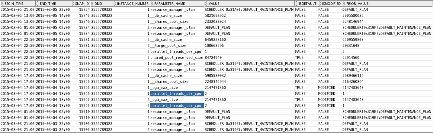
Script below produces a list of changes to System parameter values, indicating when a parameter was changed and from which value into which value. It does not filter out cache re-sizing operations, or resource manager plan changes. Both would be easy to exclude, but I’d rather see those global changes listed as well.
Note: This script below should only be executed if your site has a license for the Oracle Diagnostics pack (or Tuning pack), since it reads from AWR.
WITH
all_parameters AS (
SELECT snap_id,
       dbid,
       instance_number,
       parameter_name,
       value,
       isdefault,
       ismodified,
       lag(value) OVER (PARTITION BY dbid, instance_number, parameter_hash ORDER BY snap_id) prior_value
  FROM dba_hist_parameter
)
SELECT TO_CHAR(s.begin_interval_time, 'YYYY-MM-DD HH24:MI') begin_time,
       TO_CHAR(s.end_interval_time, 'YYYY-MM-DD HH24:MI') end_time,
       p.snap_id,
       p.dbid,
       p.instance_number,
       p.parameter_name,
       p.value,
       p.isdefault,
       p.ismodified,
       p.prior_value
  FROM all_parameters p,
       dba_hist_snapshot s
 WHERE p.value != p.prior_value
   AND s.snap_id = p.snap_id
   AND s.dbid = p.dbid
   AND s.instance_number = p.instance_number
 ORDER BY
       s.begin_interval_time DESC,
       p.dbid,
       p.instance_number,
       p.parameter_name
/
Sample output follows, where we can see a parameter affecting Degree of Parallelism was changed. This is just to illustrate its use. Enjoy this new free script! It is now part of edb360.
Free script to generate a Line Chart on HTML
Performance Metrics are easier to digest if visualized trough some Line Charts. OEM, eDB360, eAdam and other tools use them. If you already have a SQL Statement that provides the Performance Metrics you care about, and just need to generate a Line Chart for them, you can easily create a CSV file and open it with MS-Excel. But if you want to build an HTML Report out of your SQL, that is a bit harder, unless you use existing technologies. Tools like eDB360 and eAdam use Google Charts as a mechanism to easily generate such Charts. A peer asked me if we could have such functionality stand-alone, and that challenged me to create and share it.
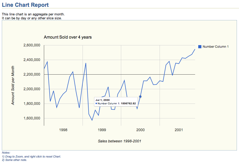
This HTML Line Chart Report above was created with script line_chart.sql shown below. The actual chart, which includes Zoom functionality on HTML can be downloaded from this Dropbox location. Feel free to use this line_chart.sql script as a template to display your Performance Metrics. It can display several series into one Chart (example above shows only one), and by reviewing code below you will find out how easy it is to adjust to your own needs. Chart above was created using a simple query against the Oracle Sample Schema SH, but the actual use could be Performance Metrics or any other Application time series.
Script
SET TERM OFF HEA OFF LIN 32767 NEWP NONE PAGES 0 FEED OFF ECHO OFF VER OFF LONG 32000 LONGC 2000 WRA ON TRIMS ON TRIM ON TI OFF TIMI OFF ARRAY 100 NUM 20 SQLBL ON BLO . RECSEP OFF;
PRO
DEF report_title = "Line Chart Report";
DEF report_abstract_1 = "<br>This line chart is an aggregate per month.";
DEF report_abstract_2 = "<br>It can be by day or any other slice size.";
DEF report_abstract_3 = "";
DEF report_abstract_4 = "";
DEF chart_title = "Amount Sold over 4 years";
DEF xaxis_title = "Sales between 1998-2001";
--DEF vaxis_title = "Amount Sold per Hour";
--DEF vaxis_title = "Amount Sold per Day";
DEF vaxis_title = "Amount Sold per Month";
DEF vaxis_baseline = ", baseline:2200000";
DEF chart_foot_note_1 = "<br>1) Drag to Zoom, and right click to reset Chart.";
DEF chart_foot_note_2 = "<br>2) Some other note.";
DEF chart_foot_note_3 = "";
DEF chart_foot_note_4 = "";
DEF report_foot_note = "This is a sample line chart report.";
PRO
SPO line_chart.html;
PRO <html>
PRO <!-- $Header: line_chart.sql 2014-07-27 carlos.sierra $ -->
PRO <head>
PRO <title>line_chart.html</title>
PRO
PRO <style type="text/css">
PRO body   {font:10pt Arial,Helvetica,Geneva,sans-serif; color:black; background:white;}
PRO h1     {font-size:16pt; font-weight:bold; color:#336699; border-bottom:1px solid #cccc99; margin-top:0pt; margin-bottom:0pt; padding:0px 0px 0px 0px;}
PRO h2     {font-size:14pt; font-weight:bold; color:#336699; margin-top:4pt; margin-bottom:0pt;}
PRO h3     {font-size:12pt; font-weight:bold; color:#336699; margin-top:4pt; margin-bottom:0pt;}
PRO pre    {font:8pt monospace;Monaco,"Courier New",Courier;}
PRO a      {color:#663300;}
PRO table  {font-size:8pt; border_collapse:collapse; empty-cells:show; white-space:nowrap; border:1px solid #cccc99;}
PRO li     {font-size:8pt; color:black; padding-left:4px; padding-right:4px; padding-bottom:2px;}
PRO th     {font-weight:bold; color:white; background:#0066CC; padding-left:4px; padding-right:4px; padding-bottom:2px;}
PRO td     {color:black; background:#fcfcf0; vertical-align:top; border:1px solid #cccc99;}
PRO td.c   {text-align:center;}
PRO font.n {font-size:8pt; font-style:italic; color:#336699;}
PRO font.f {font-size:8pt; color:#999999; border-top:1px solid #cccc99; margin-top:30pt;}
PRO </style>
PRO
PRO <script type="text/javascript" src="https://www.google.com/jsapi"></script>
PRO <script type="text/javascript">
PRO google.load("visualization", "1", {packages:["corechart"]})
PRO google.setOnLoadCallback(drawChart)
PRO
PRO function drawChart() {
PRO var data = google.visualization.arrayToDataTable([
/* add below more columns if needed (modify 3 places) */
PRO ['Date Column', 'Number Column 1']
/****************************************************************************************/
WITH
my_query AS (
/* query below selects one date_column and a small set of number_columns */
SELECT --TRUNC(time_id, 'HH24') date_column /* preserve the column name */
       --TRUNC(time_id, 'DD') date_column /* preserve the column name */
       TRUNC(time_id, 'MM') date_column /* preserve the column name */
       , SUM(amount_sold) number_column_1 /* add below more columns if needed (modify 3 places) */
  FROM sh.sales
 GROUP BY
       --TRUNC(time_id, 'HH24') /* aggregate per hour, but it could be any other */
       --TRUNC(time_id, 'DD') /* aggregate per day, but it could be any other */
       TRUNC(time_id, 'MM') /* aggregate per month, but it could be any other */
/* end of query */
)
/****************************************************************************************/
/* no need to modify the date column below, but you may need to add some number columns */
SELECT ', [new Date('||
       TO_CHAR(q.date_column, 'YYYY')|| /* year */
       ','||(TO_NUMBER(TO_CHAR(q.date_column, 'MM')) - 1)|| /* month - 1 */
       --','||TO_CHAR(q.date_column, 'DD')|| /* day */
       --','||TO_CHAR(q.date_column, 'HH24')|| /* hour */
       --','||TO_CHAR(q.date_column, 'MI')|| /* minute */
       --','||TO_CHAR(q.date_column, 'SS')|| /* second */
       ')'||
       ','||q.number_column_1|| /* add below more columns if needed (modify 3 places) */
       ']'
  FROM my_query q
 ORDER BY
       date_column
/
/****************************************************************************************/
PRO ]);
PRO
PRO var options = {
PRO backgroundColor: {fill: '#fcfcf0', stroke: '#336699', strokeWidth: 1},
PRO explorer: {actions: ['dragToZoom', 'rightClickToReset'], maxZoomIn: 0.1},
PRO title: '&&chart_title.',
PRO titleTextStyle: {fontSize: 16, bold: false},
PRO focusTarget: 'category',
PRO legend: {position: 'right', textStyle: {fontSize: 12}},
PRO tooltip: {textStyle: {fontSize: 10}},
PRO hAxis: {title: '&&xaxis_title.', gridlines: {count: -1}},
PRO vAxis: {title: '&&vaxis_title.' &&vaxis_baseline., gridlines: {count: -1}}
PRO }
PRO
PRO var chart = new google.visualization.LineChart(document.getElementById('chart_div'))
PRO chart.draw(data, options)
PRO }
PRO </script>
PRO </head>
PRO <body>
PRO <h1>&&report_title.</h1>
PRO &&report_abstract_1.
PRO &&report_abstract_2.
PRO &&report_abstract_3.
PRO &&report_abstract_4.
PRO <div id="chart_div" style="width: 900px; height: 500px;"></div>
PRO <font class="n">Notes:</font>
PRO <font class="n">&&chart_foot_note_1.</font>
PRO <font class="n">&&chart_foot_note_2.</font>
PRO <font class="n">&&chart_foot_note_3.</font>
PRO <font class="n">&&chart_foot_note_4.</font>
PRO <pre>
L
PRO </pre>
PRO <br>
PRO <font class="f">&&report_foot_note.</font>
PRO </body>
PRO </html>
SPO OFF;
SET HEA ON LIN 80 NEWP 1 PAGES 14 FEED ON ECHO OFF VER ON LONG 80 LONGC 80 WRA ON TRIMS OFF TRIM OFF TI OFF TIMI OFF ARRAY 15 NUM 10 NUMF "" SQLBL OFF BLO ON RECSEP WR;
eAdam
Enkitec’s Oracle AWR Data Mining Tool
 eAdam is a free tool that extracts a subset of data and metadata from an Oracle database with the objective to perform some data mining using a separate staging Oracle database. The data extracted is relevant to Performance Evaluations projects. Most of the data eAdam extracts is licensed by Oracle under the Diagnostics Pack, and some under the Tuning Pack. Therefore, in order to use this eAdam tool, the source database must be licensed to use both Oracle Packs (Tuning and Diagnostics).
To a point, eAdam is similar to eDB360; both access the Data Dictionary in order to produce some reports. The key difference is that eDB360 generates all the reports (after doing some intensive processing) at the source database, while eAdam simply extracts a set of flat files into a TAR file, using a very light-weight script, delaying all the intensive processing for a later time and on a separate staging system. This feature can be very attractive for busy systems where the amount of processing of any external monitoring tool needs to be minimized.
On the source system, eAdam only needs to execute a short script to extract the data and metadata of interest, producing a dense TAR file. On a staging system, eAdam does the heavy lifting, requiring the creation of a repository, the load of this repository and finally the computation of meaningful reports. The processing of the TAR file into the staging system is usually performed by the requestor, using a lower-level database, or a remote one.
The list of objects eAdam extracts as flat files from the source database includes the following:
dba_hist_active_sess_history
dba_hist_database_instance
dba_hist_event_histogram
dba_hist_osstat
dba_hist_parameter
dba_hist_pgastat
dba_hist_sga
dba_hist_sgastat
dba_hist_snapshot
dba_hist_sql_plan
dba_hist_sqlstat
dba_hist_sqltext
dba_hist_sys_time_model
dba_hist_sysstat
gv$active_session_history
gv$log
gv$sql_monitor
gv$sql_plan_monitor
gv$sql_plan_statistics_all
gv$sql
gv$system_parameter2
v$controlfile
v$datafile
v$tempfile
eAdam works on 10gR2, 11gR2, and on higher releases of Oracle; and it can be used on Linux or UNIX Platforms. It has not been tested on Windows. An eAdam sample output is available at this Dropbox location; after downloading the sample output, look for the 0001_eadam36_N_dbname_index.html file and start browsing.
Instructions – Source Database
Download the tool, uncompress the master ZIP file, and look for file eadam-master/source_system/eadam_extract.sql. Review and execute this single and short script connecting to the source database as SYS or DBA. Locate the TAR file produced, and send it to the requestor.
Be aware that the TAR file produced by the extraction process can be large, so be sure you execute this extract script from a directory with at least 10 GBs of free space. Common sizes of this TAR file range between 100 MBs and 1 GB. Execution time for this extraction process may exceed 1 hour, depending on the size of the Data Dictionary.
Instructions – Staging Database
Be sure you have both the eAdam tool (eadam-master.zip) and the TAR file produced on a source system. Your staging database can be of equal, higher or lower release level than the source, but equal or higher is recommended. The Platform can be the same or different.
To install, load and report on the staging database, proceed with the following steps:
- Create on the staging system a file directory available to Oracle for read and write. Most probably you want to create this directory connecting to OS as Oracle and create a new directory like /home/oracle/eadam-master. Put in there the content of the eadam-master.zip file.
- Create the eAdam repository on the staging database. This step is needed only one time. Follow instructions from the eadam_readme.txt. Basically you need to execute eadam-master/stage_system/eadam_install.sql connected as SYS. This script asks for 4 parameters: Tablespace names for permanent and temporary schema objects, and the username and password of the new eAdam account. For the username I recommend eadam, but you can use any valid name.
- Load the data contained in the TAR file into the database. To do this you need first to copy the TAR file into the eadam-master/stage_system sub-directory and execute next the stage_system/eadam_load.sql script while on the stage_system sub-directory, and connecting as SYS. This script asks for 4 parameters. Pass first the directory path of your stage_system sub-directory, for example /home/oracle/eadam-master/stage_system (this sub-directory must contain the TAR file). Pass next the username and password of your eadam account as you created them. Pass last the name of the TAR file to be loaded into the database.
- The load process performs some data transformations and it produces at the end an output similar to eDB360 but smaller in content. After you review the eAdam output, you may decide to generate new output for shorter time series, in such case use the eadam-master/stage_system/eadam_report.sql connecting as the eadam user. This reporting process asks for 3 parameters. Pass the EADAM_SEQ_ID which identifies your particular load (a list of values is displayed), then pass the range of dates using format YYYY-MM-DD/HH24:MI, for example 2014-07-27/17:33.
Download
EADAM @ GitHub is available as free software. You can see its eadam_readme.txt, license.txt or any other piece of the tool before downloading it. Use this link eadam-master.zip to actually download eAdam as a compressed file.
Feedback
Please post your feedback about this eAdam tool at this blog, or send and email directly to the tool author: Carlos Sierra.
eDB360
An Oracle Database 360-degree View
 eDB360 is a free tool that executes on an Oracle database and produces a compressed file which includes a large set of small Reports. This set of Reports provides a 360-degree view of an Oracle Database. eDB360 is mostly used for one of the following 3 reasons, listed here in order of frequency of use: 1) Keystone of an Oracle database Health-Check. 2) Kick-off for an Oracle database Performance Evaluation. 3) High-level view of System Resources demand and utilization for an Oracle database Sizing and Provisioning project.
Usually, Developers, Sys Admins and Consultants are not given open access to a database in a Production environment. This eDB360 free tool helps approved users to become familiar with an Oracle database in a non-intrusive way. Without installing anything on the database, the eDB360 tool connects to an Oracle database and produces a large set of flat files that can be reviewed offline while using an HTML browser or a Text editor.
eDB360 can be executed by someone with very limited access to an Oracle database (i.e. a Developer, Sys Admin or Consultant with just query access to the Data Dictionary views); or if executed by an authorized DBA, there is no actual need to provide any additional access to the Oracle database to the party requesting eDB360.
eDB360 works on 10gR2, 11gR2, and on higher releases of Oracle; and it can be used on Linux or UNIX Platforms. It has not been tested on Windows.
Instructions
Download the eDB360 tool and review the readme.md file included. Uncompress the master ZIP file on the Database Server of interest. Navigate to the main (master) directory and execute script edb360.sql connected as SYS or any other account with access to the Data Dictionary views (a DBA account is not required but it is preferred).
Execution time for eDB360 may exceed 1 hour, depending on the size of the Data Dictionary. And the size of the output may reach 1 GB, so be sure you execute this tool from a file system directory with at least 1 GB or free space. Common sizes of the output range between 10 and 100 MB.
eDB360 has only one required execution parameter:
- Oracle Pack License: A big portion of the information presented by eDB360 comes from Oracle’s Automatic Workload Repository (AWR), and AWR is licensed by Oracle under the Diagnostics Pack. A small part of the output of eDB360 comes from the SQL Monitoring repository, which is part of the Oracle Tuning Pack. This parameter accepts one of 3 values: “T”, “D” or “N”. If you database is licensed under the Oracle Tuning Pack, enter then the value of “T”. If your database is not licensed to use the Oracle Tuning Pack but it is licensed to use the Oracle Diagnostics Pack, enter “D” then. If your site is not licensed on any of these two Oracle Packs, enter “N” then. Be aware that a value of “N” reduces substantially the content and value of the output. Thus the preferred parameter value is “T” (Oracle Tuning Pack).
Sample
# unzip edb360-master.zip
# cd edb360-master
# sqlplus / as sysdba
SQL> @edb360.sql T
Download
eDB360, now part of SQLdb360, is available as free-to-use software. You can see its readme.md, license.txt or any other piece of the tool before downloading it.
Feedback
Please post your feedback about this eDB360 tool at this blog, or send and email directly to the tool author: Carlos Sierra.
